Ch17 因果生存分析¶

Causal Survial Analysis

内容摘要¶

在前面的章节中，我们一直关注有关在特定时间点发生的治疗对结果影响的因果问题。例如，我们估计了1982年戒烟对体重增加的影响。但是，许多因果关系问题涉及到treatment effects on the time until the occurrence of an event of interest. 例如，我们可能想要估算the causal effect of smoking cessation on the time until death, whenever death occurs. 这是生存分析的一个例子。

使用“生存”一词并不意味着所关注的事件必定是死亡。术语“生存分析”或等效术语 “failure time analysis” 适用于事件发生时间的任何分析，其中事件可能是死亡，婚姻，监禁，癌症，流感感染等。生存分析需要一些特殊的考虑和技巧，因为许多人的失败时间可能在研究结束后发生，因此未知。本章 outlines basic techniques for survival analysis in the simplified setting of time-fixed treatments.

17.1 Hazards and risks¶

17.2 From hazards to risks¶

17.3 Why censoring matter¶

17.4 IP weighting of marginal structural model¶

When the treated and the untreated are not exchangeable, a direct contrast of their survival curves cannot be endowed with a causal interpretation.

17.5 The parametric g-formula¶

In the previous section we estimated the survival curve under treatment and under no treatment in the entire study population via IP weighting. To do so, we adjusted for \(L\) and assumed exchangeability, positivity, and consistency. Another method to estimate the marginal survival curves under those assumptions is standardization based on parametric models, that is, the parametric g-formula.

17.6 G-estimation of structural nested models¶

The previous sections describe causal contrasts that compare survivals, or risks, under different levels of treatment \(A\). The survival was computed from haz- ards estimated by logistic regression models. This approach is feasible when the analytic method is IP weighting of marginal structural models or the para- metric g-formula, but not when the method is g-estimation of structural nested models. As explained in Chapter 14, structural nested models are models for conditional causal contrasts (e.g., the difference or ratio of covariate-specific means under different treatment levels), not for the components of those con- trasts (e.g., each of the means under different treatment levels). Therefore we cannot estimate survivals or hazards using a structural nested model.

Programs¶

[1]:

%matplotlib inline

[2]:

import warnings
warnings.filterwarnings('ignore')

[3]:

import numpy as np
import pandas as pd
import statsmodels.api as sm
import matplotlib.pyplot as plt
from tqdm import tqdm

[4]:

nhefs_all = pd.read_excel('NHEFS.xls')

WARNING *** OLE2 inconsistency: SSCS size is 0 but SSAT size is non-zero

[5]:

for col in ['age', 'wt71', 'smokeintensity', 'smokeyrs']:
    nhefs_all['{}^2'.format(col)] = nhefs_all[col] * nhefs_all[col]

[6]:

nhefs_all['one'] = 1

[7]:

edu_dummies = pd.get_dummies(nhefs_all.education, prefix='edu')
exercise_dummies = pd.get_dummies(nhefs_all.exercise, prefix='exercise')
active_dummies = pd.get_dummies(nhefs_all.active, prefix='active')

nhefs_all = pd.concat(
    [nhefs_all, edu_dummies, exercise_dummies, active_dummies],
    axis=1
)

[8]:

nhefs_all.shape

[8]:

(1629, 80)

Check the number that died during follow-up

[9]:

death = nhefs_all.death
print("      # died: {:>4}".format(death.sum()))
print("# didn't die: {:>4}".format((1 - nhefs_all.death).sum()))

      # died:  318
# didn't die: 1311

Number of deaths for untreated and treated

[10]:

nhefs_all.groupby('qsmk').agg({'death': 'sum'}).T

[10]:

qsmk	0	1
death	216	102

Check the first and last dates of recorded death

[11]:

date_death = 10000 * nhefs_all.yrdth + 100 * nhefs_all.modth + nhefs_all.dadth
date_death = pd.to_datetime(date_death, format="%y%m%d")
print("first death: {}".format(date_death.min().strftime("%b %d, %Y")))
print(" last death: {}".format(date_death.max().strftime("%b %d, %Y")))

first death: Jan 08, 1983
 last death: Dec 12, 1992

Program 17.1¶

Add longevity and survived to the data set

The longevity will be the number of months of follow-up lived until death. If the individual did not die, the value is set to the number of follow-up months, 120.

[12]:

nhefs_all['longevity'] = (nhefs_all.yrdth - 83) * 12 + nhefs_all.modth - 1
nhefs_all.longevity.replace(np.NaN, 120, inplace=True)

[13]:

nhefs_all['survived'] = 1 - nhefs_all.death

Percent of survived at month 120 for untreated and treated

[14]:

nhefs_all.groupby('qsmk').agg(
    {'survived': lambda col: '{:>0.1f}%'.format(100 * col.mean())}
).T

[14]:

qsmk	0	1
survived	82.0%	76.2%

Log-rank test: “a common statistical test to compare survival curves”, pg 211 margin

[15]:

chisq, pvalue = sm.duration.survdiff(
    nhefs_all.longevity,
    nhefs_all.death,
    nhefs_all.qsmk
)

print('log-rank test p-value: {:>0.3f}'.format(pvalue))

log-rank test p-value: 0.005

Survival curve plot

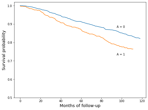
This plot is constructed by iterating through months and measuring the fraction of longevity values greater than that month. Those fraction values are the survival curve values.

[16]:

longevity0 = nhefs_all.longevity.loc[nhefs_all.qsmk == 0]
longevity1 = nhefs_all.longevity.loc[nhefs_all.qsmk == 1]

[17]:

# non-quitters
max0 = int(longevity0[longevity0 < 120].max())  # max longevity for non-quitters
surv_curve_0 = [
    (longevity0 > i).sum() / longevity0.shape[0]  # fraction of longevities greather than current month i
    for i in range(max0)
]

# quitters
max1 = int(longevity1[longevity1 < 120].max())  # max longevity for quitters
surv_curve_1 = [
    (longevity1 > i).sum() / longevity1.shape[0]  # fraction of longevities greather than current month i
    for i in range(max1)
]

[18]:

fig, ax = plt.subplots(figsize=(8, 6))

ax.plot(surv_curve_0)
ax.plot(surv_curve_1)
ax.set_ylim(0.5, 1.02)
ax.set_xlabel('Months of follow-up', fontsize=14)
ax.set_ylabel('Survival probability', fontsize=14)
ax.text(95, 0.88, 'A = 0')
ax.text(95, 0.73, 'A = 1');

Hazard at 120 months for treated

[19]:

numer = (longevity1 == 119).sum()
denom = (longevity1 > 118).sum()
print('{}/{} = {:>0.2f}%'.format(numer, denom, numer * 100.0 / denom))

0/326 = 0.00%

Hazard at 120 months for untreated

[20]:

numer = (longevity0 == 119).sum()
denom = (longevity0 > 118).sum()
print('{}/{} = {:>0.2f}%'.format(numer, denom, numer * 100.0 / denom))

1/986 = 0.10%

The description of the curves above is different from the book. The book describes calculating the hazard by “dividing the number of cases during the interval \(k\) by the number of individuals alive at the end of the interval \(k - 1\)” and, from pg 212,

\[\text{Pr}[D_k = 0] = \prod_{m=1}^k \text{Pr}[D_m =0 | D_{m-1} = 0]\]

“That is, the survival at \(k\) equals the product of one minus the hazard at all previous times.”

I’ll show that you get (roughly) the same values for the survival curve for qsmk = 0.

[21]:

hazard0 = [
    (longevity0 == i).sum() / (longevity0 >= i - 1).sum()
    for i in range(max0)
]

Survival curves will be calculated from hazard values multiple times throughout the notebook, so I’ll make a function

[22]:

def survival_curve(hazard):
    survival = [1 - hazard[0]]
    for i in range(1, len(hazard)):
        survival.append((1 - hazard[i]) * survival[i - 1])
    return survival

[23]:

survival0_v2 = survival_curve(hazard0)

[24]:

surv_curve_0[:5]

[24]:

[1.0, 1.0, 1.0, 0.9991673605328892, 0.9983347210657785]

[25]:

survival0_v2[:5]

[25]:

[1.0, 1.0, 1.0, 0.9991673605328892, 0.9983354143542607]

[26]:

max_diff = np.abs([a - b for a, b in zip(surv_curve_0, survival0_v2)]).max()
print("maximum difference between methods: {:>0.2e}".format(max_diff))

maximum difference between methods: 2.87e-04

This difference is likely due to a propagation of rounding errors, and probably wouldn’t be visible on the plot

Program 17.2¶

Create the person-time format

The following function will be used throughout this notebook to create the person-time format

[27]:

def person_time_format(data):
    # This works for the current data only; it requires the data
    # have `longevity` and `death` columns.

    # accumulate rows in a dict, then convert the dict to DataFrame;
    # the dict will contain each column of the input data, plus
    # `time`, which keeps track of month within individual, and
    # `event`, a 0/1 indicator of death for each month
    newrows = {name: [] for name in data.columns}
    newrows.update({'time': [], 'event': []})

    for _, row in data.iterrows():
        # n_mos: a zero for each month of `longevity`
        # and then a zero/one to indicate death afterwards
        n_mos = int(row.longevity + row.death)
        for name in data.columns:
            newrows[name].extend([row[name]] * n_mos)
        newrows['time'].extend(range(n_mos))
        newrows['event'].extend([0] * n_mos)
        if row.death:
            newrows['event'][-1] = 1

    return pd.DataFrame(newrows)

[28]:

pt_data = person_time_format(nhefs_all)

[29]:

pt_data.shape

[29]:

(176764, 84)

“An easy way to parametrically estimate the hazards is to fit a logistic regression model …”, pg 213

[30]:

model = sm.Logit.from_formula(
    'event ~ qsmk + qsmk:time + qsmk:np.power(time, 2) + time + np.power(time, 2)',
    data=pt_data
)
res = model.fit()

Optimization terminated successfully.
         Current function value: 0.013100
         Iterations 11

[31]:

res.summary().tables[1]

[31]:

	coef	std err	z	P>\|z\|	[0.025	0.975]
Intercept	-6.9956	0.231	-30.291	0.000	-7.448	-6.543
qsmk	0.3355	0.397	0.845	0.398	-0.443	1.114
qsmk:time	0.0121	0.015	0.804	0.422	-0.017	0.042
qsmk:np.power(time, 2)	-0.0002	0.000	-1.293	0.196	-0.000	8.31e-05
time	0.0196	0.008	2.329	0.020	0.003	0.036
np.power(time, 2)	-0.0001	6.69e-05	-1.878	0.060	-0.000	5.47e-06

Create predictions for each time point, for both qsmk == 0 and qsmk == 1

[32]:

A0_pred = res.predict(
    pd.DataFrame({'time': list(range(120)), 'qsmk': [0] * 120})
)
A1_pred = res.predict(
    pd.DataFrame({'time': list(range(120)), 'qsmk': [1] * 120})
)

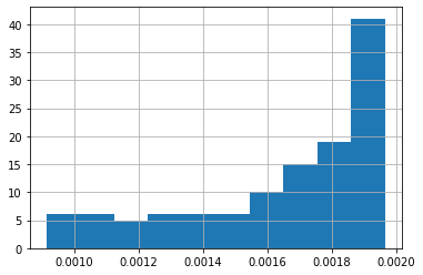
Just a quick look at the values of A0_pred

[33]:

A0_pred.hist();

Create the model-based survival curves, and recreate Figure 17.2

The survival_curve function below was defined in cell 22 above. For explanation, see the text between cells 20 and 21.

[34]:

model_surv_0 = survival_curve(A0_pred)
model_surv_1 = survival_curve(A1_pred)

[35]:

fig, ax = plt.subplots(figsize=(8, 6))

ax.plot(model_surv_0)
ax.plot(model_surv_1)
ax.set_ylim(0.5, 1.02)
ax.set_xlabel('Months of follow-up', fontsize=14)
ax.set_ylabel('Survival probability', fontsize=14)
ax.text(95, 0.88, 'A = 0')
ax.text(95, 0.73, 'A = 1');

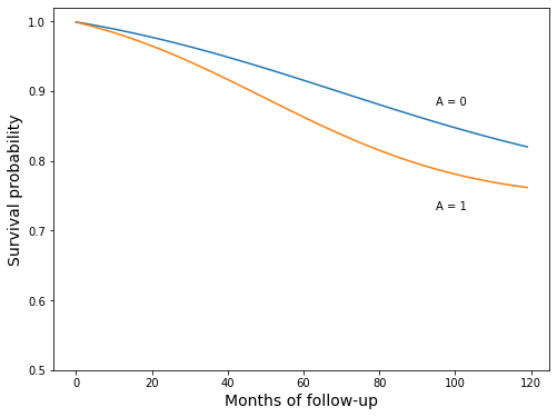
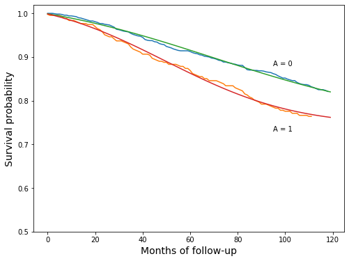
“These curves are a smooth version of those in Figure 17.1”, pg 213

Plot the new parametric version and the previous nonparametric version together, just to see how well they line up

[36]:

fig, ax = plt.subplots(figsize=(8, 6))

ax.plot(surv_curve_0)
ax.plot(surv_curve_1)

ax.plot(model_surv_0)
ax.plot(model_surv_1)

ax.set_ylim(0.5, 1.02)
ax.set_xlabel('Months of follow-up', fontsize=14)
ax.set_ylabel('Survival probability', fontsize=14)
ax.text(95, 0.88, 'A = 0')
ax.text(95, 0.73, 'A = 1');

Program 17.3¶

“The estimation of IP weighted survival curves has two steps”

“First, we estimate the stabilized IP weights \(SW^A\)”, pg 217

We’ll once again borrow a function from Chapter 12 to create IP weights

[37]:

def logit_ip_weights(y, X):
    """
    Create IP weights from logistic regression

    Parameters
    ----------
    y : Pandas Series
    X : Pandas DataFrame

    Returns
    -------
    Numpy array of IP weights

    """
    model = sm.Logit(y, X)
    res = model.fit()
    weights = np.zeros(X.shape[0])
    weights[y == 1] = res.predict(X.loc[y == 1])
    weights[y == 0] = 1 - res.predict(X.loc[y == 0])
    return weights

[38]:

X = nhefs_all[[
    'one', 'sex', 'race', 'edu_2', 'edu_3', 'edu_4', 'edu_5',
    'exercise_1', 'exercise_2', 'active_1', 'active_2',
    'age', 'age^2', 'wt71', 'wt71^2',
    'smokeintensity', 'smokeintensity^2', 'smokeyrs', 'smokeyrs^2'
]]

[39]:

ip_denom = logit_ip_weights(nhefs_all.qsmk, X)

Optimization terminated successfully.
         Current function value: 0.542264
         Iterations 6

[40]:

pr_qsmk = nhefs_all.qsmk.mean()

ip_numer = np.zeros(ip_denom.shape[0])
ip_numer[nhefs_all.qsmk == 0] = 1 - pr_qsmk
ip_numer[nhefs_all.qsmk == 1] = pr_qsmk

[41]:

ip_weights = ip_numer / ip_denom

[42]:

print('Stabilized weights')
print(' min   mean    max')
print('------------------')
print('{:>04.2f}   {:>04.2f}   {:>04.2f}'.format(
    ip_weights.min(),
    ip_weights.mean(),
    ip_weights.max()
))

Stabilized weights
 min   mean    max
------------------
0.33   1.00   4.21

“Second, using the person-time format, we fit a harzards model like the one described in Section 17.2, except that individuals are weighted by their estimated \(SW^A\)”, pg 217

So, recreate the person-time dataset, but with weights, and fit the model. We can create the person-time format by adding the IP weights to the dataset, and using the function person_time_format from above. Since that function expands every column into the person-time format, it’ll handle the weights too.

[43]:

nhefs_all['weight'] = ip_weights

[44]:

pt_data = person_time_format(nhefs_all)

[45]:

model = sm.GLM.from_formula(
    'event ~ qsmk + qsmk:time + qsmk:np.power(time, 2) + time + np.power(time, 2)',
    freq_weights=pt_data.weight,
    family=sm.families.Binomial(),
    data=pt_data
)
res = model.fit()
res.summary()

[45]:

Generalized Linear Model Regression Results
Dep. Variable:	event	No. Observations:	176764
Model:	GLM	Df Residuals:	176922.33
Model Family:	Binomial	Df Model:	5
Link Function:	logit	Scale:	1.0000
Method:	IRLS	Log-Likelihood:	-2313.1
Date:	Wed, 22 Jan 2020	Deviance:	4626.2
Time:	21:46:47	Pearson chi2:	1.76e+05
No. Iterations:	10
Covariance Type:	nonrobust

	coef	std err	z	P>\|z\|	[0.025	0.975]
Intercept	-6.8970	0.221	-31.241	0.000	-7.330	-6.464
qsmk	-0.1794	0.440	-0.408	0.683	-1.042	0.683
qsmk:time	0.0189	0.016	1.155	0.248	-0.013	0.051
qsmk:np.power(time, 2)	-0.0002	0.000	-1.556	0.120	-0.000	5.47e-05
time	0.0189	0.008	2.345	0.019	0.003	0.035
np.power(time, 2)	-0.0001	6.4e-05	-1.846	0.065	-0.000	7.31e-06

Plotting the curves is the same as last plot

[46]:

A0_pred = res.predict(
    pd.DataFrame({'time': list(range(120)), 'qsmk': [0] * 120})
)
A1_pred = res.predict(
    pd.DataFrame({'time': list(range(120)), 'qsmk': [1] * 120})
)

The survival_curve function below was defined in cell 22 above. For explanation, see the text between cells 20 and 21.

[47]:

surv_ip_0 = survival_curve(A0_pred)
surv_ip_1 = survival_curve(A1_pred)

[48]:

fig, ax = plt.subplots(figsize=(8, 6))

ax.plot(surv_ip_0)
ax.plot(surv_ip_1)
ax.set_ylim(0.5, 1.02)
ax.set_xlabel('Months of follow-up', fontsize=14)
ax.set_ylabel('Survival probability', fontsize=14)
ax.text(95, 0.88, 'A = 0')
ax.text(95, 0.76, 'A = 1');

Plot the curves on top of the curves from the previous model, to see how they’ve changed

[49]:

fig, ax = plt.subplots(figsize=(8, 6))

ax.plot(model_surv_0, linestyle=":", c="C0")
ax.plot(model_surv_1, linestyle=":", c="C1")

ax.plot(surv_ip_0, c="C0")
ax.plot(surv_ip_1, c="C1")

ax.set_ylim(0.5, 1.02)
ax.set_xlabel('Months of follow-up', fontsize=14)
ax.set_ylabel('Survival probability', fontsize=14)
ax.text(95, 0.88, 'A = 0')
ax.text(95, 0.74, 'A = 1');

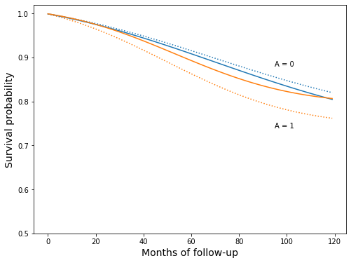
[50]:

print('survival estimates')
print('     smoking cessation: {:>0.1f}%'.format(surv_ip_1[-1] * 100))
print('  no smoking cessation: {:>0.1f}%'.format(surv_ip_0[-1] * 100))

survival estimates
     smoking cessation: 80.7%
  no smoking cessation: 80.5%

Create 500 boostrap samples to get confidence intervals

[51]:

def model_results(boot_data):
    model = sm.GLM.from_formula(
        'event ~ qsmk + qsmk:time + qsmk:np.power(time, 2) + time + np.power(time, 2)',
        freq_weights=boot_data.weight,
        family=sm.families.Binomial(),
        data=boot_data
    )
    results = model.fit()
    return results

[52]:

def month_preds(results):
    A0_pred = results.predict(
        pd.DataFrame({'time': list(range(120)), 'qsmk': [0] * 120})
    )
    A1_pred = results.predict(
        pd.DataFrame({'time': list(range(120)), 'qsmk': [1] * 120})
    )
    return A0_pred, A1_pred

[53]:

def survival_difference(boot_data):
    results = model_results(boot_data)
    A0_pred, A1_pred = month_preds(results)
    surv_ip_0 = survival_curve(A0_pred)
    surv_ip_1 = survival_curve(A1_pred)
    min_diff = min(s1 - s0 for s1, s0 in zip(surv_ip_1, surv_ip_0))
    end_diff = surv_ip_1[-1] - surv_ip_0[-1]
    return min_diff, end_diff

The next cell will take a while to run

[54]:

min_diff_samples = []
end_diff_samples = []
nrows = pt_data.shape[0]
for i in tqdm(range(500)):
    boot_data = pt_data.sample(nrows, replace=True, axis=0)
    min_diff, end_diff = survival_difference(boot_data)
    min_diff_samples.append(min_diff)
    end_diff_samples.append(end_diff)

100%|██████████| 500/500 [02:26<00:00,  3.41it/s]

[55]:

estimate = (surv_ip_1[-1] - surv_ip_0[-1]) * 100
ci_lo, ci_hi = np.percentile(end_diff_samples, q=[2.5, 97.5]) * 100

print('difference in final survival probability')
print('  est   CI')
print(' {:>0.1f}%   ({:>0.1f}, {:>0.1f})'.format(estimate, ci_lo, ci_hi))

difference in final survival probability
  est   CI
 0.2%   (-5.0, 4.2)

[56]:

estimate = min(s1 - s0 for s1, s0 in zip(surv_ip_1, surv_ip_0)) * 100
ci_lo, ci_hi = np.percentile(min_diff_samples, q=[2.5, 97.5]) * 100

print('largest difference in survival probability')
print('   est   CI')
print(' {:>0.1f}%   ({:>0.1f}, {:>0.1f})'.format(estimate, ci_lo, ci_hi))

largest difference in survival probability
   est   CI
 -1.9%   (-6.2, 0.1)

The previous two confidence intervals differ from the book’s, but they also change from run to run

Program 17.4¶

The steps will be similar to Program 13.3, with calculation of survival curves similar to the previous program. However, survival curves will be estimated for each individual, and the final curves will be averages of those curves

outcome modeling, on the original data (aka “block 1”)
prediction on expanded dataset per individual, see below)
- block 2: a copy of the dataset with qsmk set to zero
- block 3: a copy of the dataset with qsmk set to one
create the survival curves from the predictions, per individual, see below
average the individual curves to get marginal survival curves

Step 1

[57]:

model = sm.GLM.from_formula(
    'event ~ qsmk + qsmk:time + qsmk:I(time ** 2) + time + I(time ** 2) + sex'
    '+ race + age + I(age**2) + C(education) + smokeintensity + I(smokeintensity ** 2)'
    '+ smokeyrs + I(smokeyrs ** 2) + C(exercise) + C(active) + wt71 + I(wt71 ** 2)'
    '+ smkintensity82_71',
    family=sm.families.Binomial(),
    data=pt_data
)
res = model.fit()

[58]:

res.summary()

[58]:

Generalized Linear Model Regression Results
Dep. Variable:	event	No. Observations:	176764
Model:	GLM	Df Residuals:	176739
Model Family:	Binomial	Df Model:	24
Link Function:	logit	Scale:	1.0000
Method:	IRLS	Log-Likelihood:	-2092.9
Date:	Wed, 22 Jan 2020	Deviance:	4185.7
Time:	21:49:17	Pearson chi2:	1.74e+05
No. Iterations:	11
Covariance Type:	nonrobust

	coef	std err	z	P>\|z\|	[0.025	0.975]
Intercept	-9.2724	1.379	-6.723	0.000	-11.976	-6.569
C(education)[T.2.0]	-0.1401	0.157	-0.895	0.371	-0.447	0.167
C(education)[T.3.0]	-0.4335	0.153	-2.841	0.005	-0.733	-0.134
C(education)[T.4.0]	-0.2350	0.279	-0.842	0.400	-0.782	0.312
C(education)[T.5.0]	-0.3750	0.239	-1.571	0.116	-0.843	0.093
C(exercise)[T.1.0]	-0.1469	0.179	-0.820	0.412	-0.498	0.204
C(exercise)[T.2.0]	0.1504	0.176	0.854	0.393	-0.195	0.496
C(active)[T.1.0]	0.1601	0.130	1.232	0.218	-0.095	0.415
C(active)[T.2.0]	0.2294	0.188	1.222	0.222	-0.139	0.597
qsmk	-0.0596	0.415	-0.143	0.886	-0.874	0.755
qsmk:time	0.0149	0.015	0.987	0.324	-0.015	0.044
qsmk:I(time ** 2)	-0.0002	0.000	-1.367	0.172	-0.000	7.39e-05
time	0.0227	0.008	2.690	0.007	0.006	0.039
I(time ** 2)	-0.0001	6.71e-05	-1.750	0.080	-0.000	1.41e-05
sex	-0.4368	0.141	-3.101	0.002	-0.713	-0.161
race	0.0524	0.173	0.302	0.763	-0.288	0.392
age	0.0875	0.059	1.481	0.139	-0.028	0.203
I(age ** 2)	-8.128e-05	0.001	-0.149	0.882	-0.001	0.001
smokeintensity	0.0016	0.014	0.114	0.909	-0.026	0.030
I(smokeintensity ** 2)	7.182e-05	0.000	0.301	0.764	-0.000	0.001
smokeyrs	0.0168	0.031	0.547	0.584	-0.043	0.077
I(smokeyrs ** 2)	5.28e-05	0.000	0.124	0.901	-0.001	0.001
wt71	-0.0622	0.019	-3.270	0.001	-0.100	-0.025
I(wt71 ** 2)	0.0004	0.000	3.584	0.000	0.000	0.001
smkintensity82_71	0.0017	0.007	0.259	0.795	-0.011	0.014

Steps 2 & 3

The model gives the information for constructing conditional survival curves.

As the text says, “we can use this model to estimate the survival curves under treatment and no treatment for white men aged 61, with college education, low levels of exercise, etc. However, our goal is estimating the marginal, not the conditional”, pg 218

To get the marginal survival curves, we create conditional curves and average them. To do this, we create a full person-time set for each individual twice, once with qsmk equal to zero, and once with qsmk equal to one. Then we’ll create the survival curves for each individual, and average by time.

To create the individual person-time sets, we’ll go row-by-row through the original data, set death to zero and longevity to 120, i.e. survived through end of follow-up, and set qsmk to zero or one.

We’ll use two arrays to carry all of the survival curves, fill it in for each individual, then average the array.

[59]:

survivals_qsmk0 = np.zeros((nhefs_all.shape[0], 120))
survivals_qsmk1 = np.zeros((nhefs_all.shape[0], 120))

The survival_curve function below was defined in cell 22 above. For explanation, see the text between cells 20 and 21.

[60]:

# fill in the individual survival curves
for i, (_, row) in enumerate(nhefs_all.iterrows()):
    # the person_time_format function expects a DataFrame, so convert the
    # row to a DataFrame first
    frame = pd.DataFrame([list(row)], columns=row.index)
    frame["death"] = 0
    frame["longevity"] = 120

    # qsmk = 0 curve
    pt_block2_i = person_time_format(frame)
    pt_block2_i["qsmk"] = 0
    hazard = res.predict(pt_block2_i)
    survivals_qsmk0[i] = survival_curve(hazard)

    # qsmk = 1 curve
    pt_block3_i = pt_block2_i.copy()
    pt_block3_i["qsmk"] = 1
    hazard = res.predict(pt_block3_i)
    survivals_qsmk1[i] = survival_curve(hazard)

Step 4: Average the individual curves

[61]:

surv_gform_0 = survivals_qsmk0.mean(axis=0)
surv_gform_1 = survivals_qsmk1.mean(axis=0)

[62]:

fig, ax = plt.subplots(figsize=(8, 6))

ax.plot(surv_gform_0)
ax.plot(surv_gform_1)
ax.set_ylim(0.5, 1.02)
ax.set_xlabel('Months of follow-up', fontsize=14)
ax.set_ylabel('Survival probability', fontsize=14)
ax.text(95, 0.88, 'A = 0')
ax.text(95, 0.76, 'A = 1');

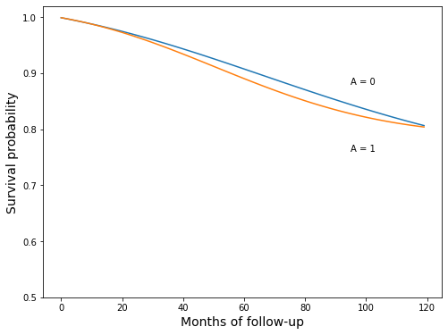
Plot these curves over the previous version, to see how they change

[63]:

fig, ax = plt.subplots(figsize=(8, 6))

ax.plot(surv_ip_0, c="C0")
ax.plot(surv_ip_1, c="C1")

ax.plot(surv_gform_0, c="C0")
ax.plot(surv_gform_1, c="C1")

ax.set_ylim(0.5, 1.02)
ax.set_xlabel('Months of follow-up', fontsize=14)
ax.set_ylabel('Survival probability', fontsize=14)
ax.text(95, 0.88, 'A = 0')
ax.text(95, 0.76, 'A = 1');

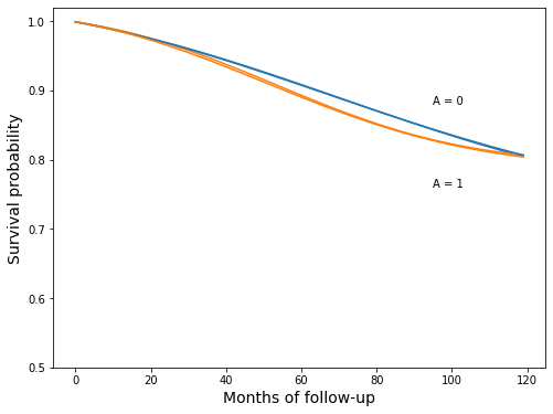
Looks like a pretty good match

Now let’s look at the mean survival curves plotted over some of the individual curves

[64]:

fig, ax = plt.subplots(figsize=(8, 6))

n_subj_tot = nhefs_all.shape[0]
for i in tqdm(range(n_subj_tot)):
    ax.plot(survivals_qsmk0[i], c="C0", alpha=0.01)
    ax.plot(survivals_qsmk1[i], c="C1", alpha=0.01)

ax.plot(surv_gform_0)
ax.plot(surv_gform_1)

ax.set_ylim(0.5, 1.02)
ax.set_xlabel('Months of follow-up', fontsize=14)
ax.set_ylabel('Survival probability', fontsize=14)
ax.text(95, 0.88, 'A = 0')
ax.text(95, 0.76, 'A = 1');

100%|██████████| 1629/1629 [00:04<00:00, 361.02it/s]

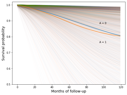
Apparently, there is a lot of variation between individuals