Ch13 标准化和参数 G-公式
内容摘要
在这一章当中 we describe how to use standardization to estimate the average causal effect of smoking cessation on body weight gain. 我们使用与上一章相同的观测数据集。尽管在第2章介绍了标准化,但我们仅将其描述为非参数方法。现在,我们将模型与标准化的结合使用,这将使我们能够 tackle high-dimensional problems with many covariates and nondichotomous treatments. 与上一章一样,我们提供计算机代码来进行分析。
在实践中,研究人员通常会在IP权重和标准化之间做出选择,作为从观测数据中获得因果效应估计的分析方法。两种方法均基于相同的可识别性条件,但基于不同的建模假设。
13.1 Standardization as an alternative to IP weighting
Goal: Estimate the causal effect of smoking cessation \(A\) on weight gain \(Y\) using standardization.
\(L\) includes the baseline variables
sex (0: male, 1: female), age (in years), race (0: white, 1: other), education (5 categories), intensity and duration of smoking (number of cigarettes per day and years of smoking), physical activity in daily life (3 categories), recreational exercise (3 categories), weight (in kg).
Subset the data as in the last chapter (though it’s not necessary to restrict on all of these columns). The standardized mean is:
13.2 Estimating the mean outcome via modeling
13.3 Standardizing the mean outcome to the confounder distribution
13.4 IP weighting or standardization?
现在,我们描述了估计平均因果效应的两种方法: IP weighting (previous chapter) and standardization (this chapter). In our smoking cessation example, both yielded almost exactly the same effect estimate. Indeed Technical Point 2.3 proved that the standardized mean equals the IP weighted mean.
It turns out that the IP weighted and the standardized mean are only exactly equal when no models are used to estimate them. Otherwise they are expected to differ. In practice some degree of misspecification is inescapable in all models, and model misspecification will introduce some bias. But the misspecification of the treatment model (IP weighting) and the outcome model (standardization) will not generally result in the same magnitude and direction of bias in the effect estimate.
It turns out that the IP weighted and the standardized mean are only exactly equal when no models are used to estimate them. Otherwise they are expected to differ. In practice some degree of misspecification is inescapable in all models, and model misspecification will introduce some bias. But the misspecification of the treatment model (IP weighting) and the outcome model (standardization) will not generally result in the same magnitude and direction of bias in the effect estimate.
13.5 How seriously do we take our estimates?
我们在本书的第一部分中回顾了平均因果效应的定义,估计平均因果效应所需的假设以及许多潜在的偏差。 这个讨论纯粹是概念性的, the data examples hypersimplistic. 一个关键信息是,在 explicitly emulating a (hypothetical) randomized experiment 时–the target trial,观测数据的因果分析更加清晰.
本章和上一章中的分析是我们从真实数据估计因果效应的首次尝试。Using both IP weighting and the parametric g-formula we estimated that the mean weight gain would have been 5.2 kg if everybody had quit smoking compared with 1.7 kg if nobody had quit smoking. 在下一章中,我们将看到获得类似的估计 when using g-estimation, outcome regression, and propensity scores.
由于每种方法的估计都是基于不同的建模假设,因此可以确保各种方法的估计的兼容性。However, observational effect estimates are always open to serious criticism. 即使我们不希望将效应估计迁移到其他总体(第4章),并且即使个体之间没有干扰,我们对目标人群的估计有效性也需要很多条件。我们将这些条件分为三类.
First, the identifiability conditions of exchangeability, positivity, and consistency (Chapter 3) need to hold 为了使得观察性研究可以看作 the target trial. The quitters and the non-quitters need to be exchangeable conditional on the 9 measured covariates \(L\) (see Fine Point 14.2). Unmeasured confounding (Chapter 7) or selection bias (Chapter 8, Fine Point 12.2) would prevent conditional exchangeability. Positivity requires that the distribution of the covariates \(L\) in the quitters fully overlaps with that in the non-quitters. Fine Point 13.1 discussed the different impact of deviations from positivity for nonparametric IP weighting and standadization. Regarding consistency, note that there are multiple versions of both quitting smoking (e.g., quitting progressively, quitting abruptly) and not quitting smoking (e.g., increasing intensity of smoking by 2 cigarettes per day, reducing intensity but not to zero). Our effect estimate corresponds to a somewhat vague hypothetical intervention in the target population that randomly assigns these versions of treatment with the same frequency as they actually have in the study population. Other hypothetical interventions might result in a different effect estimate.
Second, all variables used in the analysis need to be correctly measured. Measurement error in the treatment \(A\), the outcome \(Y\), or the confounders \(L\) will generally result in bias (Chapter 9).
Third, all models used in the analysis need to be correctly specified (Chapter 11). Suppose that the correct functional form for the continuous covariate age in the treatment model is not the parabolic curve we used but rather a curve represented by a complex polynomial. Then, even if all the confounders had been correctly measured and included in \(L\), IP weighting would not fully adjust for confounding. Model misspecification has a similar effect as measurement error in the confounders.
因果推断依赖于上述条件 which are heroic and not empirically testable. We replace the lack of data on the distribution of the counterfactual outcomes by the assumption that the above conditions are approximately met. 我们的研究越偏离这些条件,我们的效果估计就可能越有偏差。 In fact, a key step towards less casual causal inferences is the realization that the discussion should primarily revolve around each of the above assumptions. We only take our effect estimates as seriously as we take the conditions that are needed to endow them with a causal interpretation.
Programs
Setup and Imports
[1]:
%matplotlib inline

import warnings
warnings.filterwarnings('ignore')

import numpy as np
import pandas as pd
import statsmodels.api as sm
import matplotlib.pyplot as plt

nhefs_all = pd.read_excel('NHEFS.xls')
nhefs_all.shape
WARNING *** OLE2 inconsistency: SSCS size is 0 but SSAT size is non-zero
[1]:
(1629, 64)
Goal: Estimate the causal effect of smoking cessation \(A\) on weight gain \(Y\) using standardization.
\(L\) includes the baseline variables
sex (0: male, 1: female), age (in years), race (0: white, 1: other), education (5 categories), intensity and duration of smoking (number of cigarettes per day and years of smoking), physical activity in daily life (3 categories), recreational exercise (3 categories), weight (in kg).
Subset the data as in the last chapter (though it’s not necessary to restrict on all of these columns). The standardized mean is:
[2]:
restriction_cols = [
    'sex', 'age', 'race', 'wt82', 'ht', 'school', 'alcoholpy', 'smokeintensity'
]
missing = nhefs_all[restriction_cols].isnull().any(axis=1)
nhefs = nhefs_all.loc[~missing]

nhefs.shape
[2]:
(1566, 64)
[8]:
table = nhefs.groupby('qsmk').agg({'qsmk': 'count'}).T
table.index = ['count']
table
[8]:
| qsmk | 0 | 1 |
|---|---|---|
| count | 1163 | 403 |
Program 13.1
Add squared features as in chapter 12
[9]:
for col in ['age', 'wt71', 'smokeintensity', 'smokeyrs']:
    nhefs['{}^2'.format(col)] = nhefs[col] * nhefs[col]
Add constant term. We’ll call it 'one' this time.
[10]:
nhefs['one'] = 1
A column of zeros will also be useful later
[11]:
nhefs['zero'] = 0
Add dummy features
[12]:
edu_dummies = pd.get_dummies(nhefs.education, prefix='edu')
exercise_dummies = pd.get_dummies(nhefs.exercise, prefix='exercise')
active_dummies = pd.get_dummies(nhefs.active, prefix='active')

nhefs = pd.concat(
    [nhefs, edu_dummies, exercise_dummies, active_dummies],
    axis=1
)
Add interaction term
[13]:
nhefs['qsmk_x_smokeintensity'] = nhefs.qsmk * nhefs.smokeintensity
Create the model to estimate \(E[Y|A=a, C=0, L=l]\) for each combination of values of \(A\) and \(L\)
[14]:
y = nhefs.wt82_71
X = nhefs[[
    'one', 'qsmk', 'sex', 'race', 'edu_2', 'edu_3', 'edu_4', 'edu_5',
    'exercise_1', 'exercise_2', 'active_1', 'active_2',
    'age', 'age^2', 'wt71', 'wt71^2',
    'smokeintensity', 'smokeintensity^2', 'smokeyrs', 'smokeyrs^2',
    'qsmk_x_smokeintensity'
]]
[15]:
ols = sm.OLS(y, X)
res = ols.fit()
res.summary().tables[1]
[15]:
| coef | std err | t | P>|t| | [0.025 | 0.975] | |
|---|---|---|---|---|---|---|
| one | -1.5882 | 4.313 | -0.368 | 0.713 | -10.048 | 6.872 |
| qsmk | 2.5596 | 0.809 | 3.163 | 0.002 | 0.972 | 4.147 |
| sex | -1.4303 | 0.469 | -3.050 | 0.002 | -2.350 | -0.510 |
| race | 0.5601 | 0.582 | 0.963 | 0.336 | -0.581 | 1.701 |
| edu_2 | 0.7904 | 0.607 | 1.302 | 0.193 | -0.400 | 1.981 |
| edu_3 | 0.5563 | 0.556 | 1.000 | 0.317 | -0.534 | 1.647 |
| edu_4 | 1.4916 | 0.832 | 1.792 | 0.073 | -0.141 | 3.124 |
| edu_5 | -0.1950 | 0.741 | -0.263 | 0.793 | -1.649 | 1.259 |
| exercise_1 | 0.2960 | 0.535 | 0.553 | 0.580 | -0.754 | 1.346 |
| exercise_2 | 0.3539 | 0.559 | 0.633 | 0.527 | -0.742 | 1.450 |
| active_1 | -0.9476 | 0.410 | -2.312 | 0.021 | -1.752 | -0.143 |
| active_2 | -0.2614 | 0.685 | -0.382 | 0.703 | -1.604 | 1.081 |
| age | 0.3596 | 0.163 | 2.202 | 0.028 | 0.039 | 0.680 |
| age^2 | -0.0061 | 0.002 | -3.534 | 0.000 | -0.009 | -0.003 |
| wt71 | 0.0455 | 0.083 | 0.546 | 0.585 | -0.118 | 0.209 |
| wt71^2 | -0.0010 | 0.001 | -1.840 | 0.066 | -0.002 | 6.39e-05 |
| smokeintensity | 0.0491 | 0.052 | 0.950 | 0.342 | -0.052 | 0.151 |
| smokeintensity^2 | -0.0010 | 0.001 | -1.056 | 0.291 | -0.003 | 0.001 |
| smokeyrs | 0.1344 | 0.092 | 1.465 | 0.143 | -0.046 | 0.314 |
| smokeyrs^2 | -0.0019 | 0.002 | -1.209 | 0.227 | -0.005 | 0.001 |
| qsmk_x_smokeintensity | 0.0467 | 0.035 | 1.328 | 0.184 | -0.022 | 0.116 |
Look at an example prediction, for the subject with ID 24770
[16]:
example = X.loc[nhefs.seqn == 24770]
[17]:
example
[17]:
| one | qsmk | sex | race | edu_2 | edu_3 | edu_4 | edu_5 | exercise_1 | exercise_2 | ... | active_2 | age | age^2 | wt71 | wt71^2 | smokeintensity | smokeintensity^2 | smokeyrs | smokeyrs^2 | qsmk_x_smokeintensity | |
|---|---|---|---|---|---|---|---|---|---|---|---|---|---|---|---|---|---|---|---|---|---|
| 1581 | 1 | 0 | 0 | 0 | 0 | 0 | 1 | 0 | 1 | 0 | ... | 0 | 26 | 676 | 111.58 | 12450.0964 | 15 | 225 | 12 | 144 | 0 |
1 rows × 21 columns
[18]:
res.predict(example)
[18]:
1581    0.342157
dtype: float64
A quick look at mean and extremes of the predicted weight gain, across subjects
[19]:
estimated_gain = res.predict(X)
[20]:
print('   min     mean      max')
print('------------------------')
print('{:>6.2f}   {:>6.2f}   {:>6.2f}'.format(
    estimated_gain.min(),
    estimated_gain.mean(),
    estimated_gain.max()
))
   min     mean      max
------------------------
-10.88     2.64     9.88
A quick look at mean and extreme values for actual weight gain
[21]:
print('   min     mean      max')
print('------------------------')
print('{:>6.2f}   {:>6.2f}   {:>6.2f}'.format(
    nhefs.wt82_71.min(),
    nhefs.wt82_71.mean(),
    nhefs.wt82_71.max()
))
   min     mean      max
------------------------
-41.28     2.64    48.54
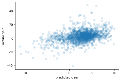
A scatterplot of predicted vs actual
[22]:
fix, ax = plt.subplots()

ax.scatter(estimated_gain, nhefs.wt82_71, alpha=0.15)
ax.set_xlabel('predicted gain')
ax.set_ylabel('actual gain');
Program 13.2
The 4 steps to the method are 1. expansion of dataset 2. outcome modeling 3. prediction 4. standardization by averaging
I am going to use a few shortcuts. “Expansion of dataset” means creating the 3 blocks described in the text. The first block (the original data) is the only one that contributes to the model, so I’ll just build the regression from the first block. The 2nd and 3rd blocks are only needed for predictions, so I’ll only create them at prediction-time.
Thus my steps will look more like 1. outcome modeling, on the original data 2. prediction on expanded dataset 3. standardization by averaging
[23]:
df = pd.DataFrame({
    'name': [
        "Rheia", "Kronos", "Demeter", "Hades", "Hestia", "Poseidon",
        "Hera", "Zeus", "Artemis", "Apollo", "Leto", "Ares", "Athena",
        "Hephaestus", "Aphrodite", "Cyclope", "Persephone", "Hermes",
        "Hebe", "Dionysus"
    ],
    'L': [0, 0, 0, 0, 0, 0, 0, 0, 1, 1, 1, 1, 1, 1, 1, 1, 1, 1, 1, 1],
    'A': [0, 0, 0, 0, 1, 1, 1, 1, 0, 0, 0, 1, 1, 1, 1, 1, 1, 1, 1, 1],
    'Y': [0, 1, 0, 0, 0, 0, 0, 1, 1, 1, 0, 1, 1, 1, 1, 1, 1, 0, 0, 0]
})

df['A_x_L'] = df.A * df.L

df['zero'] = 0
df['one'] = 1
[24]:
ols = sm.OLS(df.Y, df[['one', 'A', 'L', 'A_x_L']])
res = ols.fit()
res.summary().tables[1]
[24]:
| coef | std err | t | P>|t| | [0.025 | 0.975] | |
|---|---|---|---|---|---|---|
| one | 0.2500 | 0.255 | 0.980 | 0.342 | -0.291 | 0.791 |
| A | 1.665e-16 | 0.361 | 4.62e-16 | 1.000 | -0.765 | 0.765 |
| L | 0.4167 | 0.390 | 1.069 | 0.301 | -0.410 | 1.243 |
| A_x_L | 9.714e-17 | 0.496 | 1.96e-16 | 1.000 | -1.051 | 1.051 |
Make predictions from the second block, with all A = 0, which also makes A x L = 0.
“the average of all predicted values in the second block is precisely the standardized mean in the untreated”
[25]:
A0_pred = res.predict(df[['one', 'zero', 'L', 'zero']])
print('standardized mean: {:>0.2f}'.format(A0_pred.mean()))
standardized mean: 0.50
Make predictions from the third block, with all A = 1, which also makes A x L = L.
“To estimate the standardized mean outcome in the treated, we compute the average of all predicted values in the third block.”
[26]:
A1_pred = res.predict(df[['one', 'one', 'L', 'L']])
print('standardized mean: {:>0.2f}'.format(A1_pred.mean()))
standardized mean: 0.50
Program 13.3
We repeat the steps done above, but for the nhefs data:
outcome modeling, on the original data
prediction on expanded dataset
standardization by averaging
Step 1: Outcome modeling on the nhefs data
Note: For convenience, I’ve moved qsmk to the end of the variable list, next to qsmk_x_smokeintensity.
[27]:
y = nhefs.wt82_71
X = nhefs[[
    'one', 'sex', 'race', 'edu_2', 'edu_3', 'edu_4', 'edu_5',
    'exercise_1', 'exercise_2', 'active_1', 'active_2',
    'age', 'age^2', 'wt71', 'wt71^2',
    'smokeintensity', 'smokeintensity^2', 'smokeyrs', 'smokeyrs^2',
    'qsmk', 'qsmk_x_smokeintensity'
]]
[28]:
ols = sm.OLS(y, X)
res = ols.fit()
[29]:
res.summary().tables[1]
[29]:
| coef | std err | t | P>|t| | [0.025 | 0.975] | |
|---|---|---|---|---|---|---|
| one | -1.5882 | 4.313 | -0.368 | 0.713 | -10.048 | 6.872 |
| sex | -1.4303 | 0.469 | -3.050 | 0.002 | -2.350 | -0.510 |
| race | 0.5601 | 0.582 | 0.963 | 0.336 | -0.581 | 1.701 |
| edu_2 | 0.7904 | 0.607 | 1.302 | 0.193 | -0.400 | 1.981 |
| edu_3 | 0.5563 | 0.556 | 1.000 | 0.317 | -0.534 | 1.647 |
| edu_4 | 1.4916 | 0.832 | 1.792 | 0.073 | -0.141 | 3.124 |
| edu_5 | -0.1950 | 0.741 | -0.263 | 0.793 | -1.649 | 1.259 |
| exercise_1 | 0.2960 | 0.535 | 0.553 | 0.580 | -0.754 | 1.346 |
| exercise_2 | 0.3539 | 0.559 | 0.633 | 0.527 | -0.742 | 1.450 |
| active_1 | -0.9476 | 0.410 | -2.312 | 0.021 | -1.752 | -0.143 |
| active_2 | -0.2614 | 0.685 | -0.382 | 0.703 | -1.604 | 1.081 |
| age | 0.3596 | 0.163 | 2.202 | 0.028 | 0.039 | 0.680 |
| age^2 | -0.0061 | 0.002 | -3.534 | 0.000 | -0.009 | -0.003 |
| wt71 | 0.0455 | 0.083 | 0.546 | 0.585 | -0.118 | 0.209 |
| wt71^2 | -0.0010 | 0.001 | -1.840 | 0.066 | -0.002 | 6.39e-05 |
| smokeintensity | 0.0491 | 0.052 | 0.950 | 0.342 | -0.052 | 0.151 |
| smokeintensity^2 | -0.0010 | 0.001 | -1.056 | 0.291 | -0.003 | 0.001 |
| smokeyrs | 0.1344 | 0.092 | 1.465 | 0.143 | -0.046 | 0.314 |
| smokeyrs^2 | -0.0019 | 0.002 | -1.209 | 0.227 | -0.005 | 0.001 |
| qsmk | 2.5596 | 0.809 | 3.163 | 0.002 | 0.972 | 4.147 |
| qsmk_x_smokeintensity | 0.0467 | 0.035 | 1.328 | 0.184 | -0.022 | 0.116 |
Step 2: Prediction on expanded dataset
[30]:
block2 = nhefs[[
    'one', 'sex', 'race', 'edu_2', 'edu_3', 'edu_4', 'edu_5',
    'exercise_1', 'exercise_2', 'active_1', 'active_2',
    'age', 'age^2', 'wt71', 'wt71^2',
    'smokeintensity', 'smokeintensity^2', 'smokeyrs', 'smokeyrs^2',
    'zero', 'zero'  # qsmk = 0, and thus qsmk_x_smokeintensity = 0
]]
[31]:
block2_pred = res.predict(block2)
[32]:
block3 = nhefs[[
    'one', 'sex', 'race', 'edu_2', 'edu_3', 'edu_4', 'edu_5',
    'exercise_1', 'exercise_2', 'active_1', 'active_2',
    'age', 'age^2', 'wt71', 'wt71^2',
    'smokeintensity', 'smokeintensity^2', 'smokeyrs', 'smokeyrs^2',
    'one', 'smokeintensity'  # qsmk = 1, and thus qsmk_x_smokeintensity = smokeintensity
]]
[33]:
block3_pred = res.predict(block3)
Step 3: Standardization by averaging
[34]:
orig_mean = res.predict(X).mean()
block2_mean = block2_pred.mean()
block3_mean = block3_pred.mean()
est_diff = block3_mean - block2_mean

print('original mean prediction: {:>0.2f}'.format(orig_mean))
print()
print(' block 2 mean prediction: {:>0.2f}'.format(block2_mean))
print(' block 3 mean prediction: {:>0.2f}'.format(block3_mean))
print()
print('  causal effect estimate: {:>0.2f}'.format(est_diff))
original mean prediction: 2.64

 block 2 mean prediction: 1.76
 block 3 mean prediction: 5.27

  causal effect estimate: 3.52
Program 13.4
Use bootstrap to calculate the confidence interval on the previous estimate
If this runs too slowly, you can reduce the number of iterations in the for loop
[35]:
boot_samples = []
common_X = [
    'one', 'sex', 'race', 'edu_2', 'edu_3', 'edu_4', 'edu_5',
    'exercise_1', 'exercise_2', 'active_1', 'active_2',
    'age', 'age^2', 'wt71', 'wt71^2',
    'smokeintensity', 'smokeintensity^2', 'smokeyrs', 'smokeyrs^2'
]

for _ in range(2000):
    sample = nhefs.sample(n=nhefs.shape[0], replace=True)

    y = sample.wt82_71
    X = sample[common_X + ['qsmk', 'qsmk_x_smokeintensity']]
    block2 = sample[common_X + ['zero', 'zero']]
    block3 = sample[common_X + ['one', 'smokeintensity']]

    result = sm.OLS(y, X).fit()

    block2_pred = result.predict(block2)
    block3_pred = result.predict(block3)

    boot_samples.append(block3_pred.mean() - block2_pred.mean())
[36]:
std = np.std(boot_samples)
[37]:
lo = est_diff - 1.96 * std
hi = est_diff + 1.96 * std

print('               estimate   95% C.I.')
print('causal effect   {:>6.1f}   ({:>0.1f}, {:>0.1f})'.format(est_diff, lo, hi))
               estimate   95% C.I.
causal effect      3.5   (2.6, 4.5)
This confidence interval can be slightly different from the book values, because of bootstrap randomness
It turns out that the IP weighted and the standardized mean are only exactly equal when no models are used to estimate them. Otherwise they are expected to differ. In practice some degree of misspecification is inescapable in all models, and model misspecification will introduce some bias. But the misspecification of the treatment model (IP weighting) and the outcome model (standardization) will not generally result in the same magnitude and direction of bias in the effect estimate.
Both IP weighting and standardization are estimators of the g-formula, a general method for causal inference first described in 1986. (Part III provides a definition of the g-formula in settings with time-varying treatments.)
We say that standardization is a plug-in g-formula estimator because it simply re- places the conditional mean outcome in the g-formula by its estimates.
When, like in this chapter, those estimates come from parametric models, we refer to the method as the parametric g-formula. Because here we were only interested in the average causal effect, we only had to estimate the conditional mean outcome.
整体把握
内容简介
在这一章当中 we describe how to use standardization to estimate the average causal effect of smoking cessation on body weight gain. 我们使用与上一章相同的观测数据集。尽管在第2章介绍了标准化,但我们仅将其描述为非参数方法。现在,我们将模型与标准化的结合使用,这将使我们能够 tackle high-dimensional problems with many covariates and nondichotomous treatments.
在实践中,研究人员通常会在IP权重和标准化之间做出选择,作为从观测数据中获得因果效应估计的分析方法。两种方法均基于相同的可识别性条件,但基于不同的建模假设。
In the previous chapter we estimated the average causal effect of smoking cessation \(A\) (1: yes, 0: no) on weight gain \(Y\) (measured in kg) using IP weighting. In this chapter we will estimate the same effect using standardization. Our analyses will also be based on NHEFS data from 1629 cigarette smokers aged 25-74 years who had a baseline visit and a follow-up visit about 10 years later. Of these, 1566 individuals had their weight measured at the follow-up visit and are therefore uncensored \((C = 0)\).
Goal: Estimate the causal effect of smoking cessation \(A\) on weight gain \(Y\) using standardization.
where \(E[Y^{a, c=0}]\) is the mean weight gain that would have been observed if all individuals had received treatment level \(a\) and if no individuals had been censored. \(L\) includes the baseline variables.
sex (0: male, 1: female), age (in years), race (0: white, 1: other), education (5 categories), intensity and duration of smoking (number of cigarettes per day and years of smoking), physical activity in daily life (3 categories), recreational exercise (3 categories), weight (in kg).
Subset the data as in the last chapter (though it’s not necessary to restrict on all of these columns). The standardized mean is:
Ch13 类
用一个类来组织本章代码。
[1]:
%matplotlib inline

import warnings
warnings.filterwarnings('ignore')

from collections import OrderedDict
import numpy as np
import pandas as pd
import statsmodels.api as sm
import scipy.stats
import matplotlib.pyplot as plt
[5]:
class CH13(object):
    def __init__(self):
        self.help = "This is a demonstration for IP Weighting!"
        self.data = self.get_data()
        self.ipw_cols = None

    def get_data(self):
        nhefs_all = pd.read_excel('NHEFS.xls')
        restriction_cols = [
            'sex', 'age', 'race', 'wt82', 'ht', 'school', 'alcoholpy', 'smokeintensity'
        ]
        missing = nhefs_all[restriction_cols].isnull().any(axis=1)
        nhefs = nhefs_all.loc[~missing]
        nhefs['one'] = 1
        nhefs['zero'] = 0

        for col in ['age', 'wt71', 'smokeintensity', 'smokeyrs']:
            nhefs['{}^2'.format(col)] = nhefs[col] * nhefs[col]
        edu_dummies = pd.get_dummies(nhefs.education, prefix='edu')
        exercise_dummies = pd.get_dummies(nhefs.exercise, prefix='exercise')
        active_dummies = pd.get_dummies(nhefs.active, prefix='active')

        nhefs = pd.concat(
            [nhefs, edu_dummies, exercise_dummies, active_dummies],
            axis=1
        )

        nhefs['qsmk_x_smokeintensity'] = nhefs.qsmk * nhefs.smokeintensity
        return nhefs

    def _logit_ip_f(self, y, X):
        model = sm.Logit(y, X)
        res = model.fit()
        weights = np.zeros(X.shape[0])
        weights[y == 1] =   res.predict(X.loc[y == 1])
        weights[y == 0] = (1 - res.predict(X.loc[y == 0]))
        return weights

    def treatment_probs(self, cols=None):
        if cols is None:
            cols = ['constant', 'sex', 'race', 'age', 'age^2', 'edu_2', 'edu_3', 'edu_4', 'edu_5',
                    'smokeintensity', 'smokeintensity^2', 'smokeyrs', 'smokeyrs^2',
                    'exercise_1', 'exercise_2', 'active_1', 'active_2', 'wt71', 'wt71^2']
        self.ipw_cols = cols
        print('Confounders for IP Weight is:\n', cols)
        print()

        X_ip = self.data[cols]

        return self._logit_ip_f(self.data.qsmk, X_ip)

    def ipw(self):
        nhefs = self.data
        denoms = self.treatment_probs(self.ipw_cols)
        weights = 1 / denoms
        assert(weights.shape[0] == self.data.shape[0])
        print('Min and Max of weights:', weights.min(), weights.max())

        gee = sm.GEE(
            nhefs.wt82_71,
            nhefs[['constant', 'qsmk']],
            groups=nhefs.seqn,
            weights=weights
        )
        res = gee.fit()
        return res.summary().tables[1]

    def stabled_ipw(self):
        nhefs = self.data
        qsmk = (nhefs.qsmk == 1)
        denoms = self.treatment_probs(self.ipw_cols)
        weights = 1 / denoms
        s_weights = np.zeros(nhefs.shape[0])
        s_weights[qsmk] = qsmk.mean() * weights[qsmk]    # `qsmk` was defined a few cells ago
        s_weights[~qsmk] = (1 - qsmk).mean() * weights[~qsmk]
        print(qsmk.mean())
        gee = sm.GEE(
            nhefs.wt82_71,
            nhefs[['constant', 'qsmk']],
            groups=nhefs.seqn,
            weights=s_weights
        )
        res = gee.fit()
        return res.summary().tables[1]

    def marginal_structural_models(self):
        nhefs = self.data
        numer = self._logit_ip_f(nhefs.qsmk, nhefs[['constant', 'sex']])
        weights = 1 / self.treatment_probs()
        sw_AV = numer * weights
        nhefs['qsmk_and_female'] = nhefs.qsmk * nhefs.sex
        model = sm.WLS(
            nhefs.wt82_71,
            nhefs[['constant', 'qsmk', 'sex', 'qsmk_and_female']],
            weights=sw_AV
        )
        res = model.fit(cov_type='cluster', cov_kwds={'groups': nhefs.seqn})
        print('Marignal Structural Models 的有关变量:\n', ['constant', 'qsmk', 'sex', 'qsmk_and_female'] )
        return res.summary().tables[1]

g = CH13()
g.data
WARNING *** OLE2 inconsistency: SSCS size is 0 but SSAT size is non-zero
[5]:
| seqn | qsmk | death | yrdth | modth | dadth | sbp | dbp | sex | age | ... | edu_3 | edu_4 | edu_5 | exercise_0 | exercise_1 | exercise_2 | active_0 | active_1 | active_2 | qsmk_x_smokeintensity | |
|---|---|---|---|---|---|---|---|---|---|---|---|---|---|---|---|---|---|---|---|---|---|
| 0 | 233 | 0 | 0 | NaN | NaN | NaN | 175.0 | 96.0 | 0 | 42 | ... | 0 | 0 | 0 | 0 | 0 | 1 | 1 | 0 | 0 | 0 |
| 1 | 235 | 0 | 0 | NaN | NaN | NaN | 123.0 | 80.0 | 0 | 36 | ... | 0 | 0 | 0 | 1 | 0 | 0 | 1 | 0 | 0 | 0 |
| 2 | 244 | 0 | 0 | NaN | NaN | NaN | 115.0 | 75.0 | 1 | 56 | ... | 0 | 0 | 0 | 0 | 0 | 1 | 1 | 0 | 0 | 0 |
| 3 | 245 | 0 | 1 | 85.0 | 2.0 | 14.0 | 148.0 | 78.0 | 0 | 68 | ... | 0 | 0 | 0 | 0 | 0 | 1 | 0 | 1 | 0 | 0 |
| 4 | 252 | 0 | 0 | NaN | NaN | NaN | 118.0 | 77.0 | 0 | 40 | ... | 0 | 0 | 0 | 0 | 1 | 0 | 0 | 1 | 0 | 0 |
| ... | ... | ... | ... | ... | ... | ... | ... | ... | ... | ... | ... | ... | ... | ... | ... | ... | ... | ... | ... | ... | ... |
| 1623 | 25013 | 0 | 0 | NaN | NaN | NaN | 125.0 | 77.0 | 1 | 47 | ... | 0 | 0 | 0 | 1 | 0 | 0 | 1 | 0 | 0 | 0 |
| 1624 | 25014 | 0 | 0 | NaN | NaN | NaN | 115.0 | 66.0 | 0 | 45 | ... | 0 | 0 | 0 | 1 | 0 | 0 | 1 | 0 | 0 | 0 |
| 1625 | 25016 | 0 | 0 | NaN | NaN | NaN | 124.0 | 80.0 | 1 | 47 | ... | 0 | 0 | 0 | 1 | 0 | 0 | 1 | 0 | 0 | 0 |
| 1627 | 25032 | 0 | 0 | NaN | NaN | NaN | 171.0 | 77.0 | 0 | 68 | ... | 0 | 0 | 0 | 0 | 1 | 0 | 0 | 1 | 0 | 0 |
| 1628 | 25061 | 1 | 0 | NaN | NaN | NaN | 136.0 | 90.0 | 0 | 29 | ... | 0 | 0 | 0 | 0 | 1 | 0 | 0 | 1 | 0 | 30 |
1566 rows × 82 columns
[ ]: