SVI Part II: 条件独立性，子采样和 Amortization¶

为了对大数据使用变分推断，我们需要使用条件独立, 子采样和 Amortization等技术。

The Goal: Scaling SVI to Large Datasets

一般情况下 SVI 过程中每次更新的计算复杂度是正比于样本数，所以我们需要是用 mini-batch 的办法减少复杂度。对于具备 \(N\) 个样本的模型而言, running the model and guide and constructing the ELBO involves evaluating log pdf’s 的计算复杂度随着正比于样本数 \(N\)。这种情况在样本很多时会是一个问题，幸运的是，目标函数 ELBO 天然的支持子采样 provided that 我们的 model/guide 具有一些我们可以利用的条件独立性结构. 例如, 在 observations 在给定潜变量下条件独立时, ELBO 目标函数 \(\mathbb{E}_{q_{\phi}({\bf z})} \left [ \log p_{\theta}({\bf x}, {\bf z}) - \log q_{\phi}({\bf z}) \right]\) 中的相应对数似然有如下近似：

\[ E[\log p({\bf x}| {\bf z})] \approx \frac{1}{N}\sum_{i=1}^N \log p({\bf x}_i | {\bf z}) \approx \frac{1}{M} \sum_{i\in{\mathcal{I}_M}} \log p({\bf x}_i | {\bf z})\]

where \(\mathcal{I}_M\) is a mini-batch of indices of size \(M\) with \(M<N\) (for a discussion please see references [1,2]). 很好，问题解决了！但是我们如何在Pyro中实现这一点？

完成本章学习之后，您将理解如下的程序：

for i in range(len(data)):
    pyro.sample("obs_{}".format(i), dist.Bernoulli(f), obs=data[i])

for i in pyro.plate("data_loop", len(data)):
    pyro.sample("obs_{}".format(i), dist.Bernoulli(f), obs=data[i])

with plate('observe_data'):
    pyro.sample('obs', dist.Bernoulli(f), obs=data)

条件独立声明¶

如果我们想要在 Pyro 中使用子采样, 则首先需要确保 model 和 guide 被写成了那种可以让 Pyro 利用相关条件独立性的形式。让我们看看这究竟是如何实现的。

Pyro 提供了两种用于标记条件独立性的原语(language primitive): plate and markov. 让我们从第一个原语开始。

基本实现方法¶

Pyro.plate: 从 Sequential plate 到 Vectorized plate

让我们回到 previous tutorial 中使用的例子。为了方便起见，让我们在这里回顾 model 的主要逻辑：

def model(data):
    # sample f from the beta prior
    f = pyro.sample("latent_fairness", dist.Beta(alpha0, beta0))
    # loop over the observed data using pyro.sample with the obs keyword argument
    for i in range(len(data)):
        pyro.sample("obs_{}".format(i), dist.Bernoulli(f), obs=data[i])

对于该模型，给定潜变量 latent_fairness ，观测样本是条件独立的. 在 Pyro 中声明这种独立性的方法基本上就是使用 Pyro 的 plate 替代 Python 内置函数 range。

# 我们通过 plate 来声明给定潜变量，观测样本之间的条件独立性。
def model(data):
    # sample f from the beta prior
    f = pyro.sample("latent_fairness", dist.Beta(alpha0, beta0))
    # loop over the observed data [WE ONLY CHANGE THE NEXT LINE]
    for i in pyro.plate("data_loop", len(data)):
        pyro.sample("obs_{}".format(i), dist.Bernoulli(f), obs=data[i])

我们看到 pyro.plate 与 range 非常相似，但有一个关键区别：每次 plate 的调用需要额外指定 a unique name.

到目前为止，一切都很好。Pyro现在可以利用给定潜在随机变量下观测值的条件独立性。 But how does this actually work? 基本上，pyro.plate是使用上下文管理器(context manager)实现的。 At every execution of the body of the for loop we enter a new (conditional) independence context which is then exited at the end of the for loop body. 换句话说就是：

because each observed pyro.sample statement occurs within a different execution of the body of the for loop, Pyro marks 每个观测都是独立的。
并且这种独立性准确来说是条件独立性 given latent_fairness because latent_fairness is sampled outside of the context of data_loop.

在继续之前，让我们提一下使用 sequential plate 时要避免的一些陷阱。考虑上述代码片段的以下变体：

# WARNING 不要这样做!
my_reified_list = list(pyro.plate("data_loop", len(data)))
for i in my_reified_list:
    pyro.sample("obs_{}".format(i), dist.Bernoulli(f), obs=data[i])

这将无法得到想要的效果, since list() will enter and exit the data_loop context completely before a single pyro.sample statement is called. 类似的，用户需要注意 NOT to leak mutable computations across the boundary of the context manager, as this may lead to subtle bugs. 例如, pyro.plate 不适用于时序模型，在该模型中循环的每次执行都依赖于上一次执行; 所以时序模型中应该使用 range 或者 pyro.markov .

`plate` 向量化¶

概念上 vectorized plate 和 sequential plate 是一样的 except that it is a vectorized operation (as torch.arange is to range). 因此，它有可能实现大幅提速 compared to the explicit for loop that appears with sequential plate. Let’s see how this looks for our running example. 首先我们需要把 data 写成张量的形式:

data = torch.zeros(10)
data[0:6] = torch.ones(6)  # 6 heads and 4 tails

然后我们标记条件独立性：

# 向量化 plate 能够帮助加速后续相关计算。
with plate('observe_data'):
    pyro.sample('obs', dist.Bernoulli(f), obs=data)

让我们将其与 sequential plate 用法进行 point-by-point 比较：

这两种模式都要求用户指定 plate 唯一的 name。
注意这个代码块只引入一个观测随机变量(namely obs), since the entire tensor is considered at once.
since there is no need for an iterator in this case, 无需指定 plate context 所涉及的张量的长度。

Hint for the blew section:

for i in pyro.plate("data_loop", len(data)):
    pyro.sample("obs_{}".format(i), dist.Bernoulli(f), obs=data[i])

for i in pyro.plate("data_loop", len(data), subsample_size=5):
    pyro.sample("obs_{}".format(i), dist.Bernoulli(f), obs=data[i])

with plate('observe_data'):
    pyro.sample('obs', dist.Bernoulli(f), obs=data)

with plate('observe_data', size=10, subsample_size=5) as ind:
    pyro.sample('obs', dist.Bernoulli(f), obs=data.index_select(0, ind))

子采样¶

对于大规模数据集，每次训练只能用小批量样本进行训练，也就是 subsampling.

现在，我们知道了如何在Pyro中标记条件独立性。这本身就很有用（请参见SVI第III部分中的 dependency tracking section），但是我们也想进行子采样，以便可以对大型数据集进行 SVI 。根据 model 和 guide 的结构，Pyro支持几种进行子采样的方法。让我们一一讲解。

自动子采样 with `plate`¶

首先让我们看一下最简单的情况，在这种情况下，我们可以通过在 plate 中增加一个或者两个额外的参数来得到子采样:

for i in pyro.plate("data_loop", len(data), subsample_size=5):
    pyro.sample("obs_{}".format(i), dist.Bernoulli(f), obs=data[i])

That’s all there is to it: we just use the argument subsample_size. 每当运行model() 的时候，我们只会计算 data 5个随机抽取的样本对数似然; 此外，对数似然将自动缩放 by the appropriate factor of \(\tfrac{10}{5} = 2\). 对于向量化 plate 如何子采样? 使用方法也完全类似:

with plate('observe_data', size=10, subsample_size=5) as ind:
    pyro.sample('obs', dist.Bernoulli(f), obs=data.index_select(0, ind))

重要的是，plate现在返回一个索引ind的张量，在这种情况下，它的长度为5。请注意，除了参数subsample_size外，我们还传递了参数size，以便plate为获得张量 data 的完整大小，以便它可以计算正确的缩放因子。就像sequential plate 一样，the user is responsible for selecting the correct datapoints using the indices provided by plate.

最后, 请注意，如果数据在GPU上，则用户必须将 device 参数传递给 plate。

自定义子采样 with `plate`¶

每次 model() 运行的时候，plate 都会进行新的子采样。由于这种子采样是 stateless，因此可能会导致一些问题：对于足够大的数据集，即使经过大量的迭代，也存在不可忽略的可能性，即从未选择某些数据点。为了避免这种情况，用户可以通过 plate 的参数 subsample 来控制子采样的过程。 See the docs for details.

思考：观测数据中有缺失值的时候，模型分布中的不同变量会有数量不同的观测值，此时子采样如何进行？同一个模型分布中，不同的 plate 可以有不同的子采样大小吗？

不同分布下子采样¶

仅有局部变量时的子采样¶

我们考虑具备如下联合概率密度，也就是只有局部随机变量的 model:

\[p({\bf x}, {\bf z}) = \prod_{i=1}^N p({\bf x}_i | {\bf z}_i) p({\bf z}_i)\]

For a model with this dependency structure the scale factor introduced by subsampling scales all the terms in the ELBO by the same amount. 例如，vanilla VAE 就是这种情况。这就解释了为什么对于VAE，用户可以完全控制子采样并将 mini-batches 直接传递给 model 和 guide; plate is still used, but subsample_size and subsample are not. To see how this looks in detail, see the VAE tutorial.

同时存在局部和全局变量时的子采样¶

在掷硬币的例子中，因为唯一要抽样的是观测变量，所以 plate 只出现在 model 而没有出现在 guide 中。让我们看一个更复杂的例子，也就是 plate 出现在 model 而没有出现在 guide中. To make things simple let’s keep the discussion somewhat abstract and avoid writing a complete model and guide.

考虑一个具备如下分布的 model:

\[ p({\bf x}, {\bf z}, \beta) = p(\beta) \prod_{i=1}^N p({\bf x}_i | {\bf z}_i) p({\bf z}_i | \beta)\]

这里有 \(N\) 个观测变量 \(\{ {\bf x}_i \}\) 和 \(N\) 个局部潜变量 \(\{ {\bf z}_i \}\)，还有一个全局潜变量 \(\beta\)。我们的 gude 将被分解为

\[q({\bf z}, \beta) = q(\beta) \prod_{i=1}^N q({\bf z}_i | \beta, \lambda_i)\]

这里我们显式的引入来 \(N\) 个局部变分参数 \(\{\lambda_i \}\), while the other variational parameters are left implicit. 模型分布都指导分布都具备条件独立性结构，具体来说就是：

在模型分布中, 给定局部变量 \(\{ {\bf z}_i \}\) 观测变量 \(\{ {\bf x}_i \}\) 是条件独立的. 另外，给定 \(\beta\) 潜变量 \(\{\bf {z}_i \}\) 是条件独立的.
在指导分布中, 给定局部变分参数 \(\{\lambda_i \}\) 和全部变量 \(\beta\) 潜变量 \(\{\bf {z}_i \}\) 是条件独立的.

为了在 Pyro 中标记这些条件独立性和进行子采样, 我们需要在 model and guide 中都使用 plate. Let’s sketch out the basic logic using sequential plate (a more complete piece of code would include pyro.param statements, etc.). 首先定义模型分布:

def model(data):
    beta = pyro.sample("beta", ...) # sample the global RV
    for i in pyro.plate("locals", len(data)):
        z_i = pyro.sample("z_{}".format(i), ...)
        # compute the parameter used to define the observation
        # likelihood using the local random variable
        theta_i = compute_something(z_i)
        pyro.sample("obs_{}".format(i), dist.MyDist(theta_i), obs=data[i])

对比前面掷硬币的例子，这里 pyro.sample 同时出现在 plate loop 的里面和外面. 接下来是指导分布:

def guide(data):
    beta = pyro.sample("beta", ...) # sample the global RV
    for i in pyro.plate("locals", len(data), subsample_size=5):
        # sample the local RVs
        pyro.sample("z_{}".format(i), ..., lambda_i)

请注意，是 guide() 的索引只会被子抽样一次，Pyro 后端确保在执行 model() 期间使用相同的索引集，因此只需在 guide() 中指定 subsample_size。

More about `plate`¶

Tensor shapes and vectorized plate

在本教程中，pyro.plate 的使用仅限于相对简单的情况。 For example, none of the plates were nested inside of other plates. In order to make full use of plate, the user must be careful to use Pyro’s tensor shape semantics. For a discussion see the tensor shapes tutorial.

Amortization¶

变分自编码器(VAE)的由来

让我们再次考虑具有全局和局部潜变量的 model()，以及局部变分参数的 guide()：

\[ p({\bf x}, {\bf z}, \beta) = p(\beta) \prod_{i=1}^N p({\bf x}_i | {\bf z}_i) p({\bf z}_i | \beta) \qquad \qquad q({\bf z}, \beta) = q(\beta) \prod_{i=1}^N q({\bf z}_i | \beta, \lambda_i)\]

对于样本数 \(N\) 的情况，使用局部变分参数可以是个好方法。但是当 \(N\) 很大的时候, the fact that the space we’re doing optimization over grows with \(N\) can be a real problem. 一种避免这个问题的办法是 amortization.

这种方法是这样的。不同于引入局部变分参数 \(\lambda_i\), 我们学习一个单参数函数 \(f(\cdot)\)，定义如下形式的变分分布：

\[q(\beta) \prod_{n=1}^N q({\bf z}_i | \beta, f({\bf x}_i))\]

函数\(f(\cdot)\) （就是观测数据映射到该数据点的局部变分参数）需要足够丰富来近似后验，从而使得我们可以处理大型数据集而不必为每个样本引入一个单独的变量参数。这种方法也有其他好处： for example, during learning \(f(\cdot)\) effectively allows us to share statistical power among different datapoints. 这正是 VAE 中使用的方法。

变分自编码¶

这里使用便分布自编码器的例子查看本章所讲内容。

**Figure VAE:** **(Left)** 模型分布 **(Right)** 指导分布

完整代码¶

[1]:

import os, torch, pyro
import numpy as np
import torchvision.datasets as dset
import torch.nn as nn
import torchvision.transforms as transforms
import pyro.distributions as dist
import pyro.contrib.examples.util  # patches torchvision
from pyro.infer import SVI, Trace_ELBO
from pyro.optim import Adam
assert pyro.__version__.startswith('1.3.0')
pyro.enable_validation(True)
pyro.distributions.enable_validation(False)
pyro.set_rng_seed(0)

class Decoder(nn.Module): # 用于构建模型分布的 decoder
    def __init__(self, z_dim, hidden_dim):
        super().__init__()
        self.fc1 = nn.Linear(z_dim, hidden_dim)
        self.fc21 = nn.Linear(hidden_dim, 784)
        self.softplus = nn.Softplus()
        self.sigmoid = nn.Sigmoid()

    def forward(self, z):
        hidden = self.softplus(self.fc1(z))
        loc_img = self.sigmoid(self.fc21(hidden))
        return loc_img

class Encoder(nn.Module): # 用于构建指导分布的 encoder
    def __init__(self, z_dim, hidden_dim):
        super().__init__()
        self.fc1 = nn.Linear(784, hidden_dim)
        self.fc21 = nn.Linear(hidden_dim, z_dim)
        self.fc22 = nn.Linear(hidden_dim, z_dim)
        self.softplus = nn.Softplus()

    def forward(self, x):
        x = x.reshape(-1, 784)
        hidden = self.softplus(self.fc1(x))
        z_loc = self.fc21(hidden)
        z_scale = torch.exp(self.fc22(hidden))
        return z_loc, z_scale

class VAE(nn.Module):
    def __init__(self, z_dim=50, hidden_dim=400, use_cuda=False):
        super().__init__()
        self.encoder = Encoder(z_dim, hidden_dim)
        self.decoder = Decoder(z_dim, hidden_dim)
        if use_cuda:
            self.cuda()
        self.use_cuda = use_cuda
        self.z_dim = z_dim

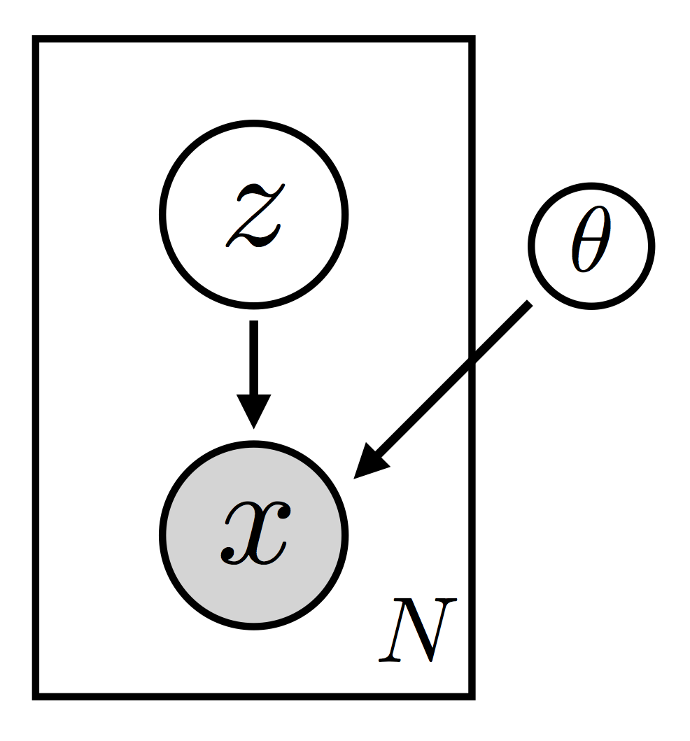
    def model(self, x): # 模型分布  p(x|z)p(z)
        pyro.module("decoder", self.decoder)
        with pyro.plate("data", x.shape[0]):
            z_loc = x.new_zeros(torch.Size((x.shape[0], self.z_dim)))
            z_scale = x.new_ones(torch.Size((x.shape[0], self.z_dim)))
            z = pyro.sample("latent", dist.Normal(z_loc, z_scale).to_event(1))
            loc_img = self.decoder.forward(z)
            pyro.sample("obs", dist.Bernoulli(loc_img).to_event(1), obs=x.reshape(-1, 784))

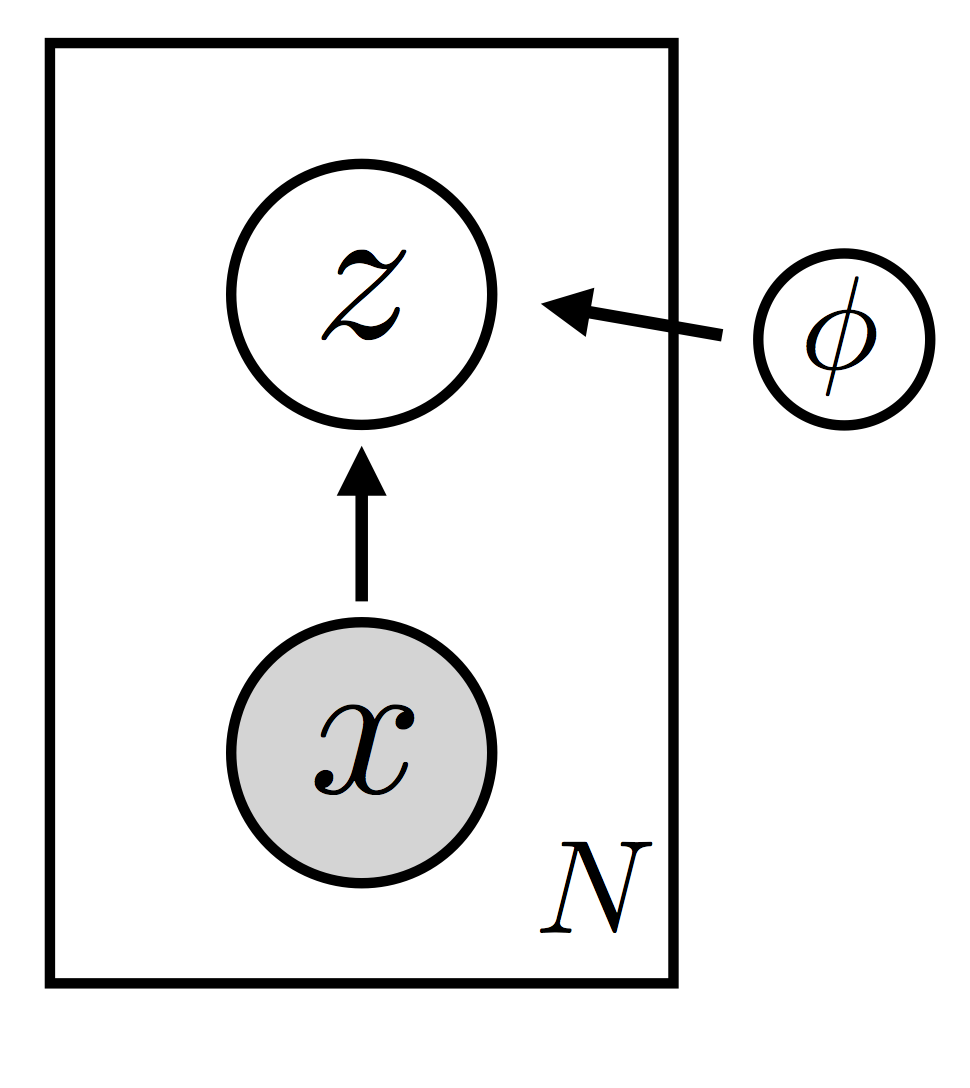
    def guide(self, x): # 指导分布 q(z|x)
        pyro.module("encoder", self.encoder)
        with pyro.plate("data", x.shape[0]):
            z_loc, z_scale = self.encoder.forward(x)
            pyro.sample("latent", dist.Normal(z_loc, z_scale).to_event(1))

    def reconstruct_img(self, x):
        z_loc, z_scale = self.encoder(x)
        z = dist.Normal(z_loc, z_scale).sample()
        loc_img = self.decoder(z) # 注意在图像空间中我们没有抽样
        return loc_img

def setup_data_loaders(batch_size=128, use_cuda=False):
    root = './data'
    download = False
    trans = transforms.ToTensor()
    train_set = dset.MNIST(root=root, train=True, transform=trans,
                           download=download)
    test_set = dset.MNIST(root=root, train=False, transform=trans)
    kwargs = {'num_workers': 1, 'pin_memory': use_cuda}
    train_loader = torch.utils.data.DataLoader(dataset=train_set,
        batch_size=batch_size, shuffle=True, **kwargs)
    test_loader = torch.utils.data.DataLoader(dataset=test_set,
        batch_size=batch_size, shuffle=False, **kwargs)
    return train_loader, test_loader

def train(svi, train_loader, use_cuda=False):
    epoch_loss = 0.
    for x, _ in train_loader:
        if use_cuda:
            x = x.cuda()
        epoch_loss += svi.step(x)
    normalizer_train = len(train_loader.dataset)
    total_epoch_loss_train = epoch_loss / normalizer_train
    return total_epoch_loss_train

def evaluate(svi, test_loader, use_cuda=False):
    test_loss = 0.
    for x, _ in test_loader:
        if use_cuda:
            x = x.cuda()
        test_loss += svi.evaluate_loss(x)
    normalizer_test = len(test_loader.dataset)
    total_epoch_loss_test = test_loss / normalizer_test
    return total_epoch_loss_test

# 模型训练
LEARNING_RATE = 1.0e-3
USE_CUDA = False
NUM_EPOCHS = 5
TEST_FREQUENCY = 5
train_loader, test_loader = setup_data_loaders(batch_size=256, use_cuda=USE_CUDA)
pyro.clear_param_store()
vae = VAE(use_cuda=USE_CUDA)
adam_args = {"lr": LEARNING_RATE}
optimizer = Adam(adam_args)
svi = SVI(vae.model, vae.guide, optimizer, loss=Trace_ELBO())

train_elbo = []
test_elbo = []
for epoch in range(NUM_EPOCHS):
    total_epoch_loss_train = train(svi, train_loader, use_cuda=USE_CUDA)
    train_elbo.append(-total_epoch_loss_train)
    print("[epoch %03d]  average training loss: %.4f" % (epoch, total_epoch_loss_train))
    if epoch % TEST_FREQUENCY == 0:
        # report test diagnostics
        total_epoch_loss_test = evaluate(svi, test_loader, use_cuda=USE_CUDA)
        test_elbo.append(-total_epoch_loss_test)
        print("[epoch %03d] average test loss: %.4f" % (epoch, total_epoch_loss_test))

[epoch 000]  average training loss: 190.9630
[epoch 000] average test loss: 155.7649
[epoch 001]  average training loss: 146.2289
[epoch 002]  average training loss: 132.9159
[epoch 003]  average training loss: 124.6936
[epoch 004]  average training loss: 119.5353

[21]:

vae.reconstruct_img(x).shape

[21]:

torch.Size([256, 784])

VAE 中条件独立，子采样和 Amortization¶

使用了 plate 来表示条件独立性。

[3]:

%psource vae.model
# 条件独立

    def model(self, x): # 模型分布  p(x|z)p(z)
        pyro.module("decoder", self.decoder)
        with pyro.plate("data", x.shape[0]):
            z_loc = x.new_zeros(torch.Size((x.shape[0], self.z_dim)))
            z_scale = x.new_ones(torch.Size((x.shape[0], self.z_dim)))
            z = pyro.sample("latent", dist.Normal(z_loc, z_scale).to_event(1))
            loc_img = self.decoder.forward(z)
            pyro.sample("obs", dist.Bernoulli(loc_img).to_event(1), obs=x.reshape(-1, 784))

You’ll need to ensure that batch_shape is carefully controlled by either trimming it down with .to_event(n) or by declaring dimensions as independent via pyro.plate.

子采样了吗？

没有进行子采样，该程序通过 setup_data_loaders 控制了每次输入的样本数是 256。（上文提到“对于VAE，用户可以完全控制子采样并将 mini-batches 直接传递给 model 和 guide; plate is still used, but subsample_size and subsample are not.”）

[2]:

train_loader, test_loader = setup_data_loaders(batch_size=256, use_cuda=USE_CUDA)
for x, _ in train_loader:
    break
print('Input shape is ', x.shape)
z = vae.encoder(x)[0]
print('encoder shape is ', z.shape)
x_ = vae.decoder.forward(z)
print('decoder shape is ', x_.shape)

Input shape is  torch.Size([256, 1, 28, 28])
encoder shape is  torch.Size([256, 50])
decoder shape is  torch.Size([256, 784])

[22]:

%psource vae.guide
# 可以看出这里没有进行子采样

    def guide(self, x): # 指导分布 q(z|x)
        pyro.module("encoder", self.encoder)
        with pyro.plate("data", x.shape[0]):
            z_loc, z_scale = self.encoder.forward(x)
            pyro.sample("latent", dist.Normal(z_loc, z_scale).to_event(1))

Amortization

VAE 是只有局部随机变量的 model:

\[p({\bf x}, {\bf z}) = \prod_{i=1}^N p_\theta({\bf x}_i | {\bf z}_i) p({\bf z}_i) \qquad \qquad q({\bf z}) = \prod_{i=1}^N q({\bf z}_i |\lambda_i)\]

where amortization \(\lambda_i = (\mu_\phi(x_i), \Sigma_\phi(x_i))\)

[23]:

%psource vae.guide
# 使用解码器进行

    def guide(self, x): # 指导分布 q(z|x)
        pyro.module("encoder", self.encoder)
        with pyro.plate("data", x.shape[0]):
            z_loc, z_scale = self.encoder.forward(x)
            pyro.sample("latent", dist.Normal(z_loc, z_scale).to_event(1))

[24]:

%psource vae.model

    def model(self, x): # 模型分布  p(x|z)p(z)
        pyro.module("decoder", self.decoder)
        with pyro.plate("data", x.shape[0]):
            z_loc = x.new_zeros(torch.Size((x.shape[0], self.z_dim)))
            z_scale = x.new_ones(torch.Size((x.shape[0], self.z_dim)))
            z = pyro.sample("latent", dist.Normal(z_loc, z_scale).to_event(1))
            loc_img = self.decoder.forward(z)
            pyro.sample("obs", dist.Bernoulli(loc_img).to_event(1), obs=x.reshape(-1, 784))

[26]:

%psource vae.decoder.forward

    def forward(self, z):
        hidden = self.softplus(self.fc1(z))
        loc_img = self.sigmoid(self.fc21(hidden))
        return loc_img

参考文献

[1] Stochastic Variational Inference, Matthew D. Hoffman, David M. Blei, Chong Wang, John Paisley

[2] Auto-Encoding Variational Bayes, Diederik P Kingma, Max Welling