SVI Part I: 随机变分推断基础
Pyro在设计时特别注意支持随机变分推断作为通用推断算法。让我们看看我们使用Pyro进行变分推断。
Table of Contents
[1]:
# Hint for the rest of this tutorial
# 完成本章学习之后,您将理解如下的程序
import math, os, torch, pyro
import torch.distributions.constraints as constraints
import pyro.distributions as dist
from pyro.optim import Adam
from pyro.infer import SVI, Trace_ELBO

assert pyro.__version__.startswith('1.3.0')
pyro.enable_validation(True)
pyro.clear_param_store()

data = []
data.extend([torch.tensor(1.0) for _ in range(6)])
data.extend([torch.tensor(0.0) for _ in range(4)])

def model(data): # 参数的先验分布是 Beta(10, 10)
    alpha0, beta0 = torch.tensor(10.0), torch.tensor(10.0)
    theta = pyro.sample("latent_fairness", dist.Beta(alpha0, beta0))
    for i in range(len(data)):
        pyro.sample("obs_{}".format(i), dist.Bernoulli(theta), obs=data[i])
def guide(data): # 参数后验分布的 guide 是 Beta(p, q), p, q 初始值为 15.0, 15.0
    alpha_q = pyro.param("alpha_q", torch.tensor(15.0), constraint=constraints.positive)
    beta_q = pyro.param("beta_q", torch.tensor(15.0), constraint=constraints.positive)
    pyro.sample("latent_fairness", dist.Beta(alpha_q, beta_q))

adam_params = {"lr": 0.0005, "betas": (0.90, 0.999)}
optimizer = Adam(adam_params)
svi = SVI(model, guide, optimizer, loss=Trace_ELBO()) # 目标函数和优化方法

n_steps = 2000
for step in range(n_steps):
    svi.step(data)
    if step % 50 == 0:
        print('.', end='')

alpha_q = pyro.param("alpha_q").item()
beta_q = pyro.param("beta_q").item()
inferred_mean = alpha_q / (alpha_q + beta_q)
factor = beta_q / (alpha_q * (1.0 + alpha_q + beta_q))
inferred_std = inferred_mean * math.sqrt(factor)
print("\nbased on the data and our prior belief, the fairness " +
      "of the coin is %.3f +- %.3f" % (inferred_mean, inferred_std))
........................................
based on the data and our prior belief, the fairness of the coin is 0.532 +- 0.090
SVI数学基础简介
我们将假设我们已经在Pyro中定义了模型(有关如何完成此操作的更多详细信息,请参见 Intro Part I)。简单回顾一下,模型就是一个带参数的随机函数 model(*args, **kwargs). 模型的每个部分都对应于某个 Pyro 语句:
观测变量 \(\Longleftrightarrow\)
pyro.samplewith theobsargument潜变量 \(\Longleftrightarrow\)
pyro.sample模型参数 \(\Longleftrightarrow\)
pyro.param
我们来看看变分推断背后的数学形式。 一个模型有观测变量 \({\bf x}\), 潜变量 \({\bf z}\) 和参数 \(\theta\). 联合概率密度如下:
我们假定组成 \(p_{\theta}({\bf x}, {\bf z})\) 的每个概率分布 \(p_i\) 具备以下的性质:
可以直接对它抽样
可以计算某点处的概率密度
关于模型参数 \(\theta\) 可微
一个直接的问题是:如何学习模型 \(p_{\theta}({\bf x}, {\bf z})\)?
在这种情况下,我们通过最大化对数证据(log evidence) 这个标准来学习一个好的模型, i.e. we want to find the value of \(\theta\) given by
其中对数证据 \(\log p_{\theta}({\bf x})\) 满足:
在一般情况下,这是一个双重困难问题. 第一个困难是因为(even for a fixed \(\theta\)) 对潜变量 \(\bf z\) 上的积分通常难以计算的。第二个困难是,即使我们知道如何计算所有 \(\theta\) 值的对数证据,也就是说对数证据是一个以参数 \(\theta\) 为自变量的函数,最大化它通常将是一个困难的非凸优化问题。
除了找到 \(\theta_{\rm{max}}\) 之外,我们还要计算潜变量 \(\bf z\) 的后验分布:
请注意,此表达式的分母就是 evidence(通常不可计算). 变分推断提供一种方案用于求解\(\theta_{\rm{max}}\) 和计算一个近似后验分布 \(p_{\theta_{\rm{max}}}({\bf z} | {\bf x})\).
总的来说,我们使用极大似然估计去求的 \(\theta_{max}\) 的思路会遇到很多麻烦。变分推断的目的是一方面估计出来联合分布的参数(也就是模型参数,得到生成模型),另外一个方面是得到后验。
指导分布
基本的想法是用一个带参指导分布 \(q_\phi(z|data)\) (\(\phi\) 被叫做变分参数) 来近似真实后验分布 \(p_\theta(z|data)\), 其中 \(q\) 被称作变分分布 (variational distribution) 。
指导分布 guide() 和模型分布一样, 它是一个包含 pyro.sample 和 pyro.param 语句的随机函数。但是指导分布不包含任何观测数据, since the guide needs to be a properly normalized distribution。注意在 Pyro 中,两个可调用对象 model() 和 guide() 必须具有相同的输入参数。
因为指导分布是潜变量后验分布 \(p_{\theta_{\rm{max}}}({\bf z} | {\bf x})\) 的近似, 那么指导分布 guide() 需要提供模型中所有潜变量的有效联合概率密度。 模型分布和指导分布中抽样语句 pyro.sample() 的变量名字必须对齐。 确切地说,如果 model() 包含随机变量 z_1
def model():
    pyro.sample("z_1", ...)
那么 guide 具备有对应的 sample statement
def guide():
    pyro.sample("z_1", ...)
两种情况下使用的分布可以不同,但是名称必须一一对应。
一旦指定了指导分布 guide() (我们在下面提供了一些明确的示例),我们就可以进行推断了。学习将就是一个优化问题 ,每次迭代都是一个 \(\theta-\phi\) space 上的梯度下降步骤,使得指导分布更加接近真实后验分布。 为此,我们需要定义适当的目标函数。
注:
因为
model = primitive r.v.(观测变量 + 潜变量) + deterministic function是一个具备观测变量的分布, 而guide给定观测变量潜变量后验分布的近似分布。在变分自编码器中,用来近似后验分布的
guide\(q_\phi(z)\) 是局部的,意味着对一个每个样本 \(x_i\),latent r.v.的后验分布 \(q_\phi(z|x_i)\) 都不相同,我们需要学习与样本个数相同数量的后验分布。
目标函数ELBO
(定义目标函数) A simple derivation (for example see reference [1]) yields what we’re after: the evidence lower bound (ELBO). The ELBO, which is a function of both \(\theta\) and \(\phi\), is defined as an expectation w.r.t. to samples from the guide:
根据假设,我们可以计算上式中期望内部对数概率 (也就是 \(\log p_{\theta}({\bf x}, {\bf z})\) 和 \(\log q_{\phi}({\bf z})\))。因为指导分布是一个可以从中采样的参数分布,所以我们可以计算 ELBO 的蒙特卡洛估计。至关重要的是 ELBO 为对数证据的下限,即对于所有的 \(\theta\) 和 \(\phi\),我们都有
因此,如果我们采取随机梯度更新来最大化 ELBO,那么我们也会 pushing the log evidence higher (in expectation)。此外,可以证明ELBO 和对数证据之间的差就是 guide 和潜变量后验分布之间的KL散度:
KL 散度是两个分布之间 “相似性” 的一个非负度量。所以对每个固定的 \(\theta\), as we take steps in \(\phi\) space that increase the ELBO, we decrease the KL divergence between the guide and the posterior, 也就是说,我们让 guide 更加接近后验分布了。 而不固定的 \(\theta\)时, we take gradient steps in both \(\theta\) and \(\phi\) space simultaneously so that the guide and model play chase, with the guide tracking a moving posterior
\(\log p_{\theta}({\bf z} | {\bf x})\)。或许有些令人惊讶是(despite the moving target),对很多不同的问题来说这个优化问题可以解决(to a suitable level of approximation).
简单来说,ELBO 是 SVI 最常见的目标函数,因为
是 \(\log p_{\theta}({\bf x})\) 的下界,所以它被叫做证据下界(evidence lower bound)。其中KL散度的定义:
See KL散度(Kullback–Leibler divergence)非负性证明
在总体思想上,变分推断很容易:我们所需要做的就是定义一个 guide() 并计算 ELBO 关于模型和指导分布参数的梯度。实际上,计算一般模型分布和指导分布的参数梯度会有一些技术难度 (see the tutorial SVI Part III for a discussion). 就本教程而言, 让我们考虑一个已解决的问题,并看看如何使用 Pyro 进行变分推理。
SVI 类
在 Pyro 中变分推断被封装在 SVI 的类中,目前只支持 ELBO 目标函数。
构建一个SVI对象,用户需要指定三个输入: model, guide 和 optimizer. 我们已经在上面讨论了模型和指导分布,并且将在下一节详细讨论优化器,因此我们现在假设手头已经有了这三个要素。To construct an instance of SVI that will do optimization via the ELBO objective, the user writes
import pyro
from pyro.infer import SVI, Trace_ELBO
svi = SVI(model, guide, optimizer, loss=Trace_ELBO())
SVI 对象有两个方法, step() 和 evaluate_loss(), that encapsulate the logic for variational learning and evaluation:
该方法
step()对其模型和指导分布中参数进行一步梯度下降,并且返回估计的损失函数 (i.e. minus the ELBO). If provided, the arguments tostep()are piped tomodel()andguide().该方法
evaluate_loss()返回估计的损失函数,但是不进行梯度下降. Just like forstep(), if provided, arguments toevaluate_loss()are piped tomodel()andguide().
对于损失函数为 ELBO 的情况,这两种方法都有可选参数 num_particles, 该参数表示样本数 used to compute the loss (in the case of evaluate_loss) and the loss and gradient (in the case of step).
optimizers
在Pyro中,model 和 guide 可以是满足如下条件的任意随机函数:
guide不能包含model中任何具有参数obs的pyro.sample语句.model和guide具备相同的输入参数(call signiture).
(动态生成的潜变量和参数问题) This presents some challenges because it means that different executions of model() and guide() may have quite different behavior, with e.g. certain latent random variables and parameters only appearing some of the time. Indeed parameters may be created dynamically during the course of inference. 也就是说 the space we’re doing optimization over, which is parameterized by \(\theta\) and \(\phi\), can grow and change dynamically.
为了支持动态参数生成,Pyro 需要为学习过程中新出现的参数动态的生成一个优化器. 幸运的是, PyTorch有一个轻量级的优化库 (see torch.optim) that can easily be repurposed for the dynamic case.
All of this is controlled by the optim.PyroOptim class, which is basically a thin wrapper around PyTorch optimizers. PyroOptim 有两个输入参数:
a constructor for PyTorch optimizers
optim_constructoranda specification of the optimizer arguments
optim_args.
总的来说, 就是在优化的过程中, 一旦某个新的参数产生, optim_constructor 就会初始化一个指定类型的优化器 with arguments given by optim_args.
Most users will probably not interact with PyroOptim directly and will instead interact with the aliases defined in optim/__init__.py. Let’s see how that goes.
有两种方法可以指定优化器参数。简单的情况是, 使用一个指定参数的固定字典 optim_args 来初始化一个 PyTorch optimizers for all the parameters:
from pyro.optim import Adam

adam_params = {"lr": 0.005, "betas": (0.95, 0.999)}
optimizer = Adam(adam_params)
第二种指定参数的方法可以实现更精细的控制。这里用户需要指定由 Pyro 唤醒的一个可调用对象,该对象将在为新生成的参数创建优化器。 该可调用对象必须有如下两个输入:
module_name: 包含参数的模块的的 Pyro name, if anyparam_name: 参数的 Pyro name
This gives the user the ability to, for example, customize learning rates for different parameters. For an example where this sort of level of control is useful, see the discussion of baselines. 下面用一个简单的例子说明这个API.
from pyro.optim import Adam

def per_param_callable(module_name, param_name):
    # 该函数与 module_name 无关,让我疑惑
    if param_name == 'my_special_parameter':
        return {"lr": 0.010}
    else:
        return {"lr": 0.001}

optimizer = Adam(per_param_callable)
这相当于告诉 Pyro 将参数 my_special_parameter 的学习速率设为 0.010,并将所有其他参数的学习速率设为0.001。
掷硬币例子
我们以一个简单的例子结束。您已获得两面硬币。您想确定硬币是否公平,即硬币以相同的频率出现正面或背面.
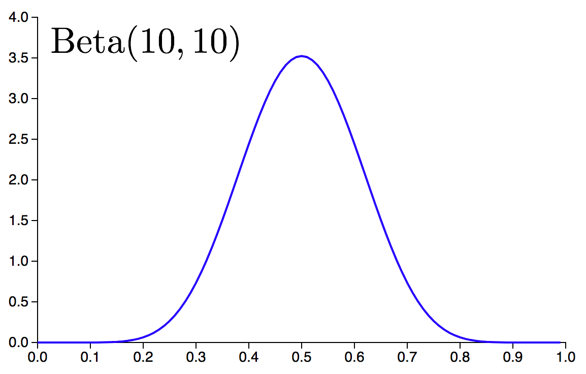
(先验分布是 \(\rm{Beta}(10,10)\)) You have a prior belief of \(\rm{Beta}(10,10)\) about the likely fairness of the coin based on two observations:
it’s a standard quarter issued by the US Mint
it’s a bit banged up from years of use
我们的模型是:
假设我们做了若干次试验,并且已经将 Measurements 收集在列表 data 中,则相应的 Pyro 模型是
import pyro.distributions as dist

def model(data):
    # define the hyperparameters that control the beta prior
    alpha0 = torch.tensor(10.0)
    beta0 = torch.tensor(10.0)
    # sample theta from the beta prior
    theta = pyro.sample("latent_fairness", dist.Beta(alpha0, beta0))
    # loop over the observed data
    for i in range(len(data)):
        # observe datapoint i using the bernoulli
        pyro.sample("obs_{}".format(i), dist.Bernoulli(theta), obs=data[i])
这里我们有一个唯一的潜变量 'latent_fairness', 它的分布是 \(\rm{Beta}(10, 10)\). Conditioned on that random variable, we observe each of the datapoints using a bernoulli likelihood. 请注意,每个观测都在 Pyro 中分配了唯一的名称.
我们的下一个任务是定义对应的指导分布 guide(),即为潜在随机变量 \(\theta\) 分配适当的变分分布。 A simple choice is to use another beta distribution parameterized by two trainable parameters \(\alpha_q\) and \(\beta_q\). Actually, in this particular case this is the ‘right’ choice, since conjugacy of the bernoulli and beta distributions means that the exact posterior is a beta distribution. In Pyro we write:
def guide(data):
    # register the two variational parameters with Pyro.
    alpha_q = pyro.param("alpha_q", torch.tensor(15.0),
                         constraint=constraints.positive)
    beta_q = pyro.param("beta_q", torch.tensor(15.0),
                        constraint=constraints.positive)
    # sample latent_fairness from the distribution Beta(alpha_q, beta_q)
    pyro.sample("latent_fairness", dist.Beta(alpha_q, beta_q))
这里有几件事情需要注意:
模型分布和指导分布中潜变量的名字必须严格一致。
model(data)和guide(data)具备相同的输入。变分参数
torch.tensor. 而pyro.param中默认requires_grad=True.我们使用
constraint=constraints.positive来实现alpha_q和beta_q在优化过程中的非负约束。
现在我们可以进行随机变分推断了。
# set up the optimizer
adam_params = {"lr": 0.0005, "betas": (0.90, 0.999)}
optimizer = Adam(adam_params)

# setup the inference algorithm
svi = SVI(model, guide, optimizer, loss=Trace_ELBO())

n_steps = 5000
# do gradient steps
for step in range(n_steps):
    svi.step(data)
注意 step() 方法中传入的 data, 它会被传入 model() 和 guide(). The only thing we’re missing at this point is some data. So let’s create some data and assemble all the code snippets above into a complete script:
[2]:
import math
import os
import torch
import torch.distributions.constraints as constraints
import pyro
from pyro.optim import Adam
from pyro.infer import SVI, Trace_ELBO
import pyro.distributions as dist

# this is for running the notebook in our testing framework
smoke_test = ('CI' in os.environ)
n_steps = 2 if smoke_test else 2000

# enable validation (e.g. validate parameters of distributions)
assert pyro.__version__.startswith('1.3.0')
pyro.enable_validation(True)

# clear the param store in case we're in a REPL
pyro.clear_param_store()

# create some data with 6 observed heads and 4 observed tails
data = []
for _ in range(6):
    data.append(torch.tensor(1.0))
for _ in range(4):
    data.append(torch.tensor(0.0))

def model(data):
    # define the hyperparameters that control the beta prior
    alpha0 = torch.tensor(10.0)
    beta0 = torch.tensor(10.0)
    # sample f from the beta prior
    theta = pyro.sample("latent_fairness", dist.Beta(alpha0, beta0))
    # loop over the observed data
    for i in range(len(data)):
        # observe datapoint i using the bernoulli likelihood
        pyro.sample("obs_{}".format(i), dist.Bernoulli(theta), obs=data[i])

def guide(data):
    # register the two variational parameters with Pyro
    # - both parameters will have initial value 15.0.
    # - because we invoke constraints.positive, the optimizer
    # will take gradients on the unconstrained parameters
    # (which are related to the constrained parameters by a log)
    alpha_q = pyro.param("alpha_q", torch.tensor(15.0),
                         constraint=constraints.positive)
    beta_q = pyro.param("beta_q", torch.tensor(15.0),
                        constraint=constraints.positive)
    # sample latent_fairness from the distribution Beta(alpha_q, beta_q)
    pyro.sample("latent_fairness", dist.Beta(alpha_q, beta_q))

# setup the optimizer
adam_params = {"lr": 0.0005, "betas": (0.90, 0.999)}
optimizer = Adam(adam_params)

# setup the inference algorithm
svi = SVI(model, guide, optimizer, loss=Trace_ELBO())

# do gradient steps
for step in range(n_steps):
    svi.step(data)
    if step % 100 == 0:
        print('.', end='')

# grab the learned variational parameters
alpha_q = pyro.param("alpha_q").item()
beta_q = pyro.param("beta_q").item()

# here we use some facts about the beta distribution
# compute the inferred mean of the coin's fairness
inferred_mean = alpha_q / (alpha_q + beta_q)
# compute inferred standard deviation
factor = beta_q / (alpha_q * (1.0 + alpha_q + beta_q))
inferred_std = inferred_mean * math.sqrt(factor)

print("\nbased on the data and our prior belief, the fairness " +
      "of the coin is %.3f +- %.3f" % (inferred_mean, inferred_std))
....................
based on the data and our prior belief, the fairness of the coin is 0.538 +- 0.089
(可以看出结果接近精确后验推断的值) This estimate is to be compared to the exact posterior mean, which in this case is given by \(16/30 = 0.5\bar{3}\). Note that the final estimate of the fairness of the coin is in between the the fairness preferred by the prior (namely \(0.50\)) and the fairness suggested by the raw empirical frequencies (\(6/10 = 0.60\)).
思考
思考问题: 优化中交替梯度下降如何手写实现?
对每个固定的 \(\theta\), as we take steps in \(\phi\) space that increase the ELBO, we decrease the KL divergence between the guide and the posterior, 也就是说,我们让 guide 更加接近后验分布了。 而不固定的 \(\theta\)时, we take gradient steps in both \(\theta\) and \(\phi\) space simultaneously so that the guide and model play chase, with the guide tracking a moving posterior \(\log p_{\theta}({\bf z} | {\bf x})\)。或许有些令人惊讶是(despite the moving
target),对很多不同的问题来说这个优化问题可以解决(to a suitable level of approximation).
下面是一个没有生成参数 \(\theta\) 的模型分布,以及具备两个变分参数 \(a, b\) 的指导分布。我们手写实现了它的梯度下降法,那么对于有生成参数 \(\theta\) 的模型分布,优化中交替梯度下降如何手写实现?
[3]:
import torch, pyro, pyro.infer, pyro.optim
import pyro.distributions as dist
import matplotlib.pyplot as plt
import numpy as np
pyro.set_rng_seed(101)
mu = 8.5

def scale(mu):
    weight = pyro.sample("weight", dist.Normal(mu, 1.0))
    return pyro.sample("measurement", dist.Normal(weight, 0.75))
conditioned_scale = pyro.condition(scale, data={"measurement": torch.tensor(9.5)})

def scale_parametrized_guide(mu):
    a = pyro.param("a", torch.tensor(mu))
    b = pyro.param("b", torch.tensor(1.))
    return pyro.sample("weight", dist.Normal(a, torch.abs(b)))

loss_fn = pyro.infer.Trace_ELBO().differentiable_loss

pyro.clear_param_store()
with pyro.poutine.trace(param_only=True) as param_capture: # 提取参数信息
    loss = loss_fn(conditioned_scale, scale_parametrized_guide, mu)
    loss.backward()
params = [site["value"].unconstrained() for site in param_capture.trace.nodes.values()]

print("Before updated:", pyro.param('a'), pyro.param('b'))

losses, a,b  = [], [], []
lr = 0.001
num_steps = 1000
# 如何手写梯度下降参数更新 for 交替梯度下降?
def step(params):
    for x in params:
        x.data = x.data - lr * x.grad
        x.grad.zero_()

for t in range(num_steps):
    with pyro.poutine.trace(param_only=True) as param_capture:
        loss = loss_fn(conditioned_scale, scale_parametrized_guide, mu)
        loss.backward()
        losses.append(loss.data)

    params = [site["value"].unconstrained() for site in param_capture.trace.nodes.values()]
    a.append(pyro.param("a").item())
    b.append(pyro.param("b").item())
    step(params)
print("After updated:", pyro.param('a'), pyro.param('b'))


plt.plot(losses)
plt.title("ELBO")
plt.xlabel("step")
plt.ylabel("loss");
print('a = ',pyro.param("a").item())
print('b = ', pyro.param("b").item())
Before updated: tensor(8.5000, requires_grad=True) tensor(1., requires_grad=True)
After updated: tensor(9.0979, requires_grad=True) tensor(0.6203, requires_grad=True)
a =  9.097911834716797
b =  0.6202840209007263
参考文献
[1] Automated Variational Inference in Probabilistic Programming, David Wingate, Theo Weber
[2] Black Box Variational Inference, Rajesh Ranganath, Sean Gerrish, David M. Blei
[3] Auto-Encoding Variational Bayes, Diederik P Kingma, Max Welling