Forecasting I: univariate, heavy tailed
This tutorial introduces the pyro.contrib.forecast module, a framework for forecasting with Pyro models. This tutorial covers only univariate models and simple likelihoods. This tutorial assumes the reader is already familiar with SVI and tensor shapes.
See also:
Summary
To create a forecasting model:
Create a subclass of the ForecastingModel class.
Implement the .model(zero_data, covariates) method using standard Pyro syntax.
Sample all time-local variables inside the self.time_plate context.
Finally call the .predict(noise_dist, prediction) method.
To train a forecasting model, create a Forecaster object.
Training can be flaky, you’ll need to tune hyperparameters and randomly restart.
Reparameterization can help learning, e.g. LocScaleReparam.
To forecast the future, draw samples from a
Forecasterobject conditioned on data and covariates.To model seasonality, use helpers periodic_features(), periodic_repeat(), and periodic_cumsum().
To model heavy-tailed data, use Stable distributions and StableReparam.
To evaluate results, use the backtest() helper or low-level loss functions.
[1]:
import torch
import pyro
import pyro.distributions as dist
import pyro.poutine as poutine
from pyro.contrib.examples.bart import load_bart_od
from pyro.contrib.forecast import ForecastingModel, Forecaster, backtest, eval_crps
from pyro.infer.reparam import LocScaleReparam, StableReparam
from pyro.ops.tensor_utils import periodic_cumsum, periodic_repeat, periodic_features
from pyro.ops.stats import quantile
import matplotlib.pyplot as plt

%matplotlib inline
assert pyro.__version__.startswith('1.3.0')
pyro.enable_validation(True)
pyro.set_rng_seed(20200221)
[2]:
dataset = load_bart_od()
print(dataset.keys())
print(dataset["counts"].shape)
print(" ".join(dataset["stations"]))
dict_keys(['stations', 'start_date', 'counts'])
torch.Size([78888, 50, 50])
12TH 16TH 19TH 24TH ANTC ASHB BALB BAYF BERY CAST CIVC COLM COLS CONC DALY DBRK DELN DUBL EMBR FRMT FTVL GLEN HAYW LAFY LAKE MCAR MLBR MLPT MONT NBRK NCON OAKL ORIN PCTR PHIL PITT PLZA POWL RICH ROCK SANL SBRN SFIA SHAY SSAN UCTY WARM WCRK WDUB WOAK
Intro to Pyro’s forecasting framework
Pyro’s forecasting framework consists of: - a ForecastingModel base class, whose .model() method can be implemented for custom forecasting models, - a Forecaster class that trains and forecasts using ForecastingModels, and - a
backtest() helper to evaluate models on a number of metrics.
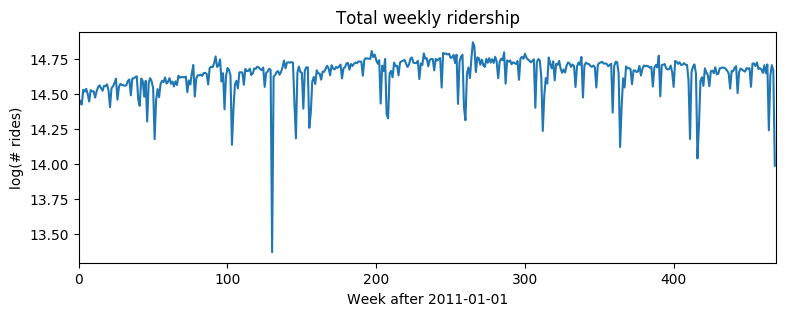
Consider a simple univariate dataset, say weekly BART train ridership aggregated over all stations in the network. This data roughly logarithmic, so we log-transform for modeling.
[3]:
T, O, D = dataset["counts"].shape
data = dataset["counts"][:T // (24 * 7) * 24 * 7].reshape(T // (24 * 7), -1).sum(-1).log()
data = data.unsqueeze(-1)
plt.figure(figsize=(9, 3))
plt.plot(data)
plt.title("Total weekly ridership")
plt.ylabel("log(# rides)")
plt.xlabel("Week after 2011-01-01")
plt.xlim(0, len(data));
Let’s start with a simple log-linear regression model, with no trend or seasonality. Note that while this example is univariate, Pyro’s forecasting framework is multivariate, so we’ll often need to reshape using .unsqueeze(-1), .expand([1]), and .to_event(1).
[4]:
# First we need some boilerplate to create a class and define a .model() method.
class Model1(ForecastingModel):
    # We then implement the .model() method. Since this is a generative model, it shouldn't
    # look at data; however it is convenient to see the shape of data we're supposed to
    # generate, so this inputs a zeros_like(data) tensor instead of the actual data.
    def model(self, zero_data, covariates):
        data_dim = zero_data.size(-1)  # Should be 1 in this univariate tutorial.
        feature_dim = covariates.size(-1)

        # The first part of the model is a probabilistic program to create a prediction.
        # We use the zero_data as a template for the shape of the prediction.
        bias = pyro.sample("bias", dist.Normal(0, 10).expand([data_dim]).to_event(1))
        weight = pyro.sample("weight", dist.Normal(0, 0.1).expand([feature_dim]).to_event(1))
        prediction = bias + (weight * covariates).sum(-1, keepdim=True)
        # The prediction should have the same shape as zero_data (duration, obs_dim),
        # but may have additional sample dimensions on the left.
        assert prediction.shape[-2:] == zero_data.shape

        # The next part of the model creates a likelihood or noise distribution.
        # Again we'll be Bayesian and write this as a probabilistic program with
        # priors over parameters.
        noise_scale = pyro.sample("noise_scale", dist.LogNormal(-5, 5).expand([1]).to_event(1))
        noise_dist = dist.Normal(0, noise_scale)

        # The final step is to call the .predict() method.
        self.predict(noise_dist, prediction)
We can now train this model by creating a Forecaster object. We’ll split the data into [T0,T1) for training and [T1,T2) for testing.
[5]:
T0 = 0              # begining
T2 = data.size(-2)  # end
T1 = T2 - 52        # train/test split
[6]:
%%time
pyro.set_rng_seed(1)
pyro.clear_param_store()
time = torch.arange(float(T2)) / 365
covariates = torch.stack([time], dim=-1)
forecaster = Forecaster(Model1(), data[:T1], covariates[:T1], learning_rate=0.1)
INFO     step    0 loss = 484401
INFO     step  100 loss = 0.609042
INFO     step  200 loss = -0.535144
INFO     step  300 loss = -0.605789
INFO     step  400 loss = -0.59744
INFO     step  500 loss = -0.596203
INFO     step  600 loss = -0.614217
INFO     step  700 loss = -0.612415
INFO     step  800 loss = -0.613236
INFO     step  900 loss = -0.59879
INFO     step 1000 loss = -0.601271
CPU times: user 5.02 s, sys: 61.6 ms, total: 5.08 s
Wall time: 5.12 s
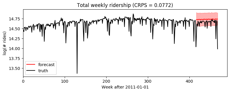
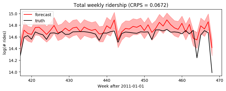
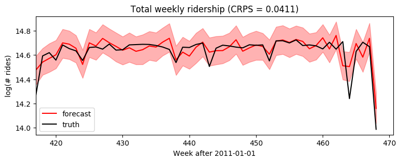
Next we can evaluate by drawing posterior samples from the forecaster, passing in full covariates but only partial data. We’ll use Pyro’s quantile() function to plot median and an 80% confidence interval. To evaluate fit we’ll use eval_crps() to compute Continuous Ranked Probability Score; this is an good metric to assess distributional fit of a heavy-tailed distribution.
[7]:
samples = forecaster(data[:T1], covariates, num_samples=1000)
p10, p50, p90 = quantile(samples, (0.1, 0.5, 0.9)).squeeze(-1)
crps = eval_crps(samples, data[T1:])
print(samples.shape, p10.shape)

plt.figure(figsize=(9, 3))
plt.fill_between(torch.arange(T1, T2), p10, p90, color="red", alpha=0.3)
plt.plot(torch.arange(T1, T2), p50, 'r-', label='forecast')
plt.plot(data, 'k-', label='truth')
plt.title("Total weekly ridership (CRPS = {:0.3g})".format(crps))
plt.ylabel("log(# rides)")
plt.xlabel("Week after 2011-01-01")
plt.xlim(0, None)
plt.legend(loc="best");
torch.Size([1000, 52, 1]) torch.Size([52])
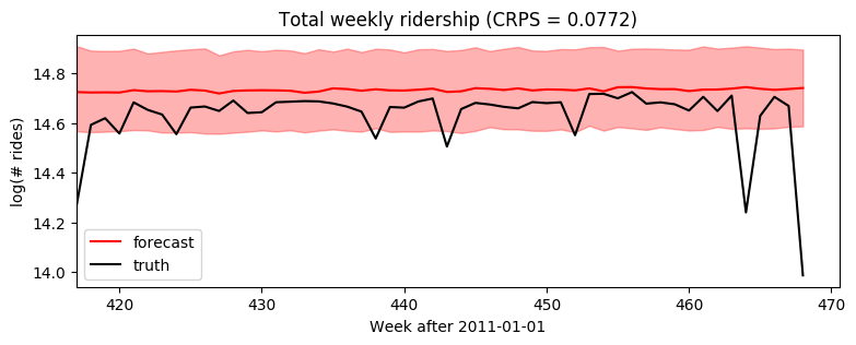
Zooming in to just the forecasted region, we see this model ignores seasonal behavior.
[8]:
plt.figure(figsize=(9, 3))
plt.fill_between(torch.arange(T1, T2), p10, p90, color="red", alpha=0.3)
plt.plot(torch.arange(T1, T2), p50, 'r-', label='forecast')
plt.plot(torch.arange(T1, T2), data[T1:], 'k-', label='truth')
plt.title("Total weekly ridership (CRPS = {:0.3g})".format(crps))
plt.ylabel("log(# rides)")
plt.xlabel("Week after 2011-01-01")
plt.xlim(T1, None)
plt.legend(loc="best");
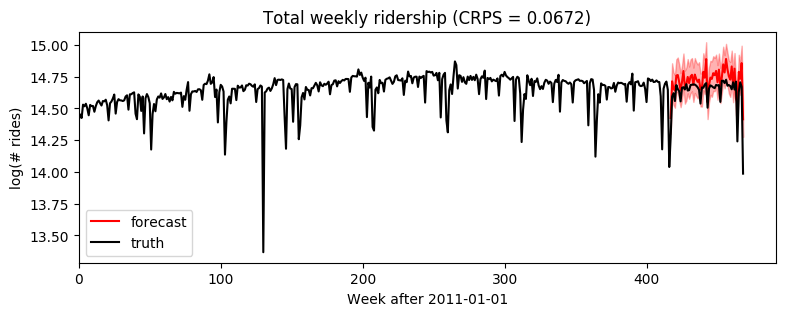
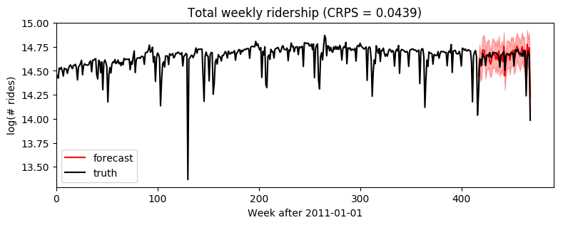
We could add a yearly seasonal component simply by adding new covariates (note we’ve already taken care in the model to handle feature_dim > 1).
[9]:
%%time
pyro.set_rng_seed(1)
pyro.clear_param_store()
time = torch.arange(float(T2)) / 365
covariates = torch.cat([time.unsqueeze(-1),
                        periodic_features(T2, 365.25 / 7)], dim=-1)
forecaster = Forecaster(Model1(), data[:T1], covariates[:T1], learning_rate=0.1)
INFO     step    0 loss = 53174.4
INFO     step  100 loss = 0.519148
INFO     step  200 loss = -0.0264822
INFO     step  300 loss = -0.314983
INFO     step  400 loss = -0.413243
INFO     step  500 loss = -0.487756
INFO     step  600 loss = -0.472516
INFO     step  700 loss = -0.595866
INFO     step  800 loss = -0.500985
INFO     step  900 loss = -0.558623
INFO     step 1000 loss = -0.589603
CPU times: user 5.74 s, sys: 88.5 ms, total: 5.83 s
Wall time: 5.89 s
[10]:
samples = forecaster(data[:T1], covariates, num_samples=1000)
p10, p50, p90 = quantile(samples, (0.1, 0.5, 0.9)).squeeze(-1)
crps = eval_crps(samples, data[T1:])

plt.figure(figsize=(9, 3))
plt.fill_between(torch.arange(T1, T2), p10, p90, color="red", alpha=0.3)
plt.plot(torch.arange(T1, T2), p50, 'r-', label='forecast')
plt.plot(data, 'k-', label='truth')
plt.title("Total weekly ridership (CRPS = {:0.3g})".format(crps))
plt.ylabel("log(# rides)")
plt.xlabel("Week after 2011-01-01")
plt.xlim(0, None)
plt.legend(loc="best");
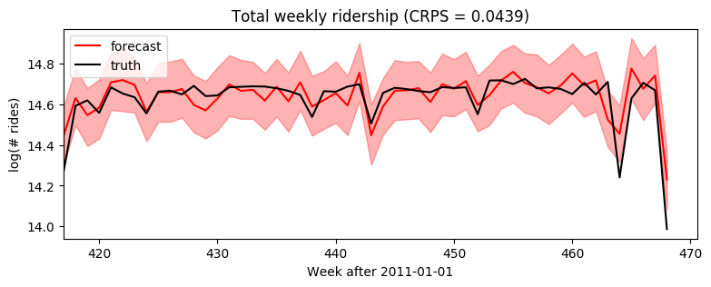
[11]:
plt.figure(figsize=(9, 3))
plt.fill_between(torch.arange(T1, T2), p10, p90, color="red", alpha=0.3)
plt.plot(torch.arange(T1, T2), p50, 'r-', label='forecast')
plt.plot(torch.arange(T1, T2), data[T1:], 'k-', label='truth')
plt.title("Total weekly ridership (CRPS = {:0.3g})".format(crps))
plt.ylabel("log(# rides)")
plt.xlabel("Week after 2011-01-01")
plt.xlim(T1, None)
plt.legend(loc="best");
Time-local random variables: self.time_plate
So far we’ve seen the ForecastingModel.model() method and self.predict(). The last piece of forecasting-specific syntax is the self.time_plate context for time-local variables. To see how this works, consider changing our global linear trend model above to a local level model. Note the poutine.reparam() handler is a general Pyro inference trick, not specific to forecasting.
[12]:
class Model2(ForecastingModel):
    def model(self, zero_data, covariates):
        data_dim = zero_data.size(-1)
        feature_dim = covariates.size(-1)
        bias = pyro.sample("bias", dist.Normal(0, 10).expand([data_dim]).to_event(1))
        weight = pyro.sample("weight", dist.Normal(0, 0.1).expand([feature_dim]).to_event(1))

        # We'll sample a time-global scale parameter outside the time plate,
        # then time-local iid noise inside the time plate.
        drift_scale = pyro.sample("drift_scale",
                                  dist.LogNormal(-20, 5).expand([1]).to_event(1))
        with self.time_plate:
            # We'll use a reparameterizer to improve variational fit. The model would still be
            # correct if you removed this context manager, but the fit appears to be worse.
            with poutine.reparam(config={"drift": LocScaleReparam()}):
                drift = pyro.sample("drift", dist.Normal(zero_data, drift_scale).to_event(1))

        # After we sample the iid "drift" noise we can combine it in any time-dependent way.
        # It is important to keep everything inside the plate independent and apply dependent
        # transforms outside the plate.
        motion = drift.cumsum(-2)  # A Brownian motion.

        # The prediction now includes three terms.
        prediction = motion + bias + (weight * covariates).sum(-1, keepdim=True)
        assert prediction.shape[-2:] == zero_data.shape

        # Construct the noise distribution and predict.
        noise_scale = pyro.sample("noise_scale", dist.LogNormal(-5, 5).expand([1]).to_event(1))
        noise_dist = dist.Normal(0, noise_scale)
        self.predict(noise_dist, prediction)
[13]:
%%time
pyro.set_rng_seed(1)
pyro.clear_param_store()
time = torch.arange(float(T2)) / 365
covariates = periodic_features(T2, 365.25 / 7)
forecaster = Forecaster(Model2(), data[:T1], covariates[:T1], learning_rate=0.1)
INFO     step    0 loss = 1.7326e+09
INFO     step  100 loss = 0.902688
INFO     step  200 loss = -0.0639999
INFO     step  300 loss = -0.102488
INFO     step  400 loss = -0.301241
INFO     step  500 loss = -0.404315
INFO     step  600 loss = -0.365754
INFO     step  700 loss = -0.429714
INFO     step  800 loss = -0.447207
INFO     step  900 loss = -0.515883
INFO     step 1000 loss = -0.519698
CPU times: user 9.11 s, sys: 66.9 ms, total: 9.18 s
Wall time: 9.21 s
[14]:
samples = forecaster(data[:T1], covariates, num_samples=1000)
p10, p50, p90 = quantile(samples, (0.1, 0.5, 0.9)).squeeze(-1)
crps = eval_crps(samples, data[T1:])

plt.figure(figsize=(9, 3))
plt.fill_between(torch.arange(T1, T2), p10, p90, color="red", alpha=0.3)
plt.plot(torch.arange(T1, T2), p50, 'r-', label='forecast')
plt.plot(data, 'k-', label='truth')
plt.title("Total weekly ridership (CRPS = {:0.3g})".format(crps))
plt.ylabel("log(# rides)")
plt.xlabel("Week after 2011-01-01")
plt.xlim(0, None)
plt.legend(loc="best");
[15]:
plt.figure(figsize=(9, 3))
plt.fill_between(torch.arange(T1, T2), p10, p90, color="red", alpha=0.3)
plt.plot(torch.arange(T1, T2), p50, 'r-', label='forecast')
plt.plot(torch.arange(T1, T2), data[T1:], 'k-', label='truth')
plt.title("Total weekly ridership (CRPS = {:0.3g})".format(crps))
plt.ylabel("log(# rides)")
plt.xlabel("Week after 2011-01-01")
plt.xlim(T1, None)
plt.legend(loc="best");
Heavy-tailed noise
Our final univariate model will generalize from Gaussian noise to heavy-tailed Stable noise. The only difference is the noise_dist which now takes two new parameters: stability determines tail weight and skew determines the relative size of positive versus negative spikes.
The Stable distribution is a natural heavy-tailed generalization of the Normal distribution, but it is difficult to work with due to its intractible density function. Pyro implements auxiliary variable methods for working with Stable distributions. To inform Pyro to use those auxiliary variable methods, we wrap the final line in poutine.reparam() effect handler
that applies the StableReparam transform to the implicit observe site named “residual”. You can use Stable distributions for other sites by specifying config={"my_site_name": StableReparam()}.
[16]:
class Model3(ForecastingModel):
    def model(self, zero_data, covariates):
        data_dim = zero_data.size(-1)
        feature_dim = covariates.size(-1)
        bias = pyro.sample("bias", dist.Normal(0, 10).expand([data_dim]).to_event(1))
        weight = pyro.sample("weight", dist.Normal(0, 0.1).expand([feature_dim]).to_event(1))

        drift_scale = pyro.sample("drift_scale", dist.LogNormal(-20, 5).expand([1]).to_event(1))
        with self.time_plate:
            with poutine.reparam(config={"drift": LocScaleReparam()}):
                drift = pyro.sample("drift", dist.Normal(zero_data, drift_scale).to_event(1))
        motion = drift.cumsum(-2)  # A Brownian motion.

        prediction = motion + bias + (weight * covariates).sum(-1, keepdim=True)
        assert prediction.shape[-2:] == zero_data.shape

        # The next part of the model creates a likelihood or noise distribution.
        # Again we'll be Bayesian and write this as a probabilistic program with
        # priors over parameters.
        stability = pyro.sample("noise_stability", dist.Uniform(1, 2).expand([1]).to_event(1))
        skew = pyro.sample("noise_skew", dist.Uniform(-1, 1).expand([1]).to_event(1))
        scale = pyro.sample("noise_scale", dist.LogNormal(-5, 5).expand([1]).to_event(1))
        noise_dist = dist.Stable(stability, skew, scale)

        # We need to use a reparameterizer to handle the Stable distribution.
        # Note "residual" is the name of Pyro's internal sample site in self.predict().
        with poutine.reparam(config={"residual": StableReparam()}):
            self.predict(noise_dist, prediction)
[17]:
%%time
pyro.set_rng_seed(2)
pyro.clear_param_store()
time = torch.arange(float(T2)) / 365
covariates = periodic_features(T2, 365.25 / 7)
forecaster = Forecaster(Model3(), data[:T1], covariates[:T1], learning_rate=0.1)
for name, value in forecaster.guide.median().items():
    if value.numel() == 1:
        print("{} = {:0.4g}".format(name, value.item()))
INFO     step    0 loss = 5.92062e+07
INFO     step  100 loss = 13.5949
INFO     step  200 loss = 3.0411
INFO     step  300 loss = 0.866627
INFO     step  400 loss = 0.362264
INFO     step  500 loss = 0.0508628
INFO     step  600 loss = -0.236901
INFO     step  700 loss = -0.290881
INFO     step  800 loss = -0.242376
INFO     step  900 loss = -0.339689
INFO     step 1000 loss = -0.33147
bias = 14.64
drift_scale = 2.173e-08
noise_stability = 1.937
noise_skew = 0.0007298
noise_scale = 0.06047
CPU times: user 19 s, sys: 97.5 ms, total: 19 s
Wall time: 19.1 s
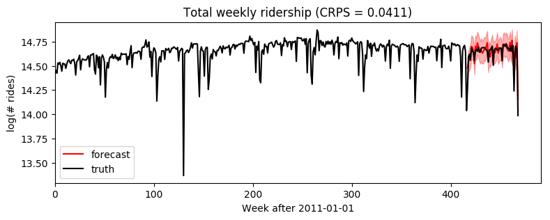
[18]:
samples = forecaster(data[:T1], covariates, num_samples=1000)
p10, p50, p90 = quantile(samples, (0.1, 0.5, 0.9)).squeeze(-1)
crps = eval_crps(samples, data[T1:])

plt.figure(figsize=(9, 3))
plt.fill_between(torch.arange(T1, T2), p10, p90, color="red", alpha=0.3)
plt.plot(torch.arange(T1, T2), p50, 'r-', label='forecast')
plt.plot(data, 'k-', label='truth')
plt.title("Total weekly ridership (CRPS = {:0.3g})".format(crps))
plt.ylabel("log(# rides)")
plt.xlabel("Week after 2011-01-01")
plt.xlim(0, None)
plt.legend(loc="best");
[19]:
plt.figure(figsize=(9, 3))
plt.fill_between(torch.arange(T1, T2), p10, p90, color="red", alpha=0.3)
plt.plot(torch.arange(T1, T2), p50, 'r-', label='forecast')
plt.plot(torch.arange(T1, T2), data[T1:], 'k-', label='truth')
plt.title("Total weekly ridership (CRPS = {:0.3g})".format(crps))
plt.ylabel("log(# rides)")
plt.xlabel("Week after 2011-01-01")
plt.xlim(T1, None)
plt.legend(loc="best");
Backtesting
To compare our Gaussian Model2 and Stable Model3 we’ll use a simple backtesting() helper. This helper by default evaluates three metrics: CRPS assesses distributional accuracy of heavy-tailed data,
MAE assesses point accuracy of heavy-tailed data, and RMSE assesses accuracy of Normal-tailed data. The one nuance here is to set warm_start=True to reduce the need for random restarts.
[20]:
%%time
pyro.set_rng_seed(1)
pyro.clear_param_store()
windows2 = backtest(data, covariates, Model2,
                    min_train_window=104, test_window=52, stride=26,
                    forecaster_options={"learning_rate": 0.1, "log_every": 1000,
                                        "warm_start": True})
INFO     Training on window [0:104], testing on window [104:156]
INFO     step    0 loss = 3534.09
INFO     step 1000 loss = 0.11251
INFO     Training on window [0:130], testing on window [130:182]
INFO     step    0 loss = 0.238584
INFO     step 1000 loss = -0.184576
INFO     Training on window [0:156], testing on window [156:208]
INFO     step    0 loss = 0.62968
INFO     step 1000 loss = -0.0259982
INFO     Training on window [0:182], testing on window [182:234]
INFO     step    0 loss = 0.195288
INFO     step 1000 loss = -0.120416
INFO     Training on window [0:208], testing on window [208:260]
INFO     step    0 loss = 0.188322
INFO     step 1000 loss = -0.18523
INFO     Training on window [0:234], testing on window [234:286]
INFO     step    0 loss = 0.0471417
INFO     step 1000 loss = -0.185852
INFO     Training on window [0:260], testing on window [260:312]
INFO     step    0 loss = 0.00251847
INFO     step 1000 loss = -0.246146
INFO     Training on window [0:286], testing on window [286:338]
INFO     step    0 loss = -0.0702055
INFO     step 1000 loss = -0.25786
INFO     Training on window [0:312], testing on window [312:364]
INFO     step    0 loss = -0.133986
INFO     step 1000 loss = -0.375242
INFO     Training on window [0:338], testing on window [338:390]
INFO     step    0 loss = -0.167895
INFO     step 1000 loss = -0.331766
INFO     Training on window [0:364], testing on window [364:416]
INFO     step    0 loss = -0.270294
INFO     step 1000 loss = -0.438097
INFO     Training on window [0:390], testing on window [390:442]
INFO     step    0 loss = -0.297009
INFO     step 1000 loss = -0.473476
INFO     Training on window [0:416], testing on window [416:468]
INFO     step    0 loss = -0.398169
INFO     step 1000 loss = -0.502486
CPU times: user 1min 51s, sys: 724 ms, total: 1min 52s
Wall time: 1min 52s
[21]:
%%time
pyro.set_rng_seed(1)
pyro.clear_param_store()
windows3 = backtest(data, covariates, Model3,
                    min_train_window=104, test_window=52, stride=26,
                    forecaster_options={"learning_rate": 0.1, "log_every": 1000,
                                        "warm_start": True})
INFO     Training on window [0:104], testing on window [104:156]
INFO     step    0 loss = 1849.22
INFO     step 1000 loss = 0.543365
INFO     Training on window [0:130], testing on window [130:182]
INFO     step    0 loss = 2.51271
INFO     step 1000 loss = 0.0757928
INFO     Training on window [0:156], testing on window [156:208]
INFO     step    0 loss = 2.6663
INFO     step 1000 loss = 0.0912818
INFO     Training on window [0:182], testing on window [182:234]
INFO     step    0 loss = 1.97279
INFO     step 1000 loss = -0.00365819
INFO     Training on window [0:208], testing on window [208:260]
INFO     step    0 loss = 1.59146
INFO     step 1000 loss = -0.0871935
INFO     Training on window [0:234], testing on window [234:286]
INFO     step    0 loss = 1.34227
INFO     step 1000 loss = -0.103136
INFO     Training on window [0:260], testing on window [260:312]
INFO     step    0 loss = 1.21624
INFO     step 1000 loss = -0.214513
INFO     Training on window [0:286], testing on window [286:338]
INFO     step    0 loss = 1.0086
INFO     step 1000 loss = -0.272347
INFO     Training on window [0:312], testing on window [312:364]
INFO     step    0 loss = 0.962262
INFO     step 1000 loss = -0.293812
INFO     Training on window [0:338], testing on window [338:390]
INFO     step    0 loss = 0.598708
INFO     step 1000 loss = -0.190582
INFO     Training on window [0:364], testing on window [364:416]
INFO     step    0 loss = 0.719034
INFO     step 1000 loss = -0.362534
INFO     Training on window [0:390], testing on window [390:442]
INFO     step    0 loss = 0.353514
INFO     step 1000 loss = -0.431448
INFO     Training on window [0:416], testing on window [416:468]
INFO     step    0 loss = 0.402931
INFO     step 1000 loss = -0.48814
CPU times: user 4min, sys: 1.07 s, total: 4min 1s
Wall time: 4min 3s
[22]:
fig, axes = plt.subplots(3, figsize=(8, 6), sharex=True)
axes[0].set_title("Gaussian versus Stable accuracy over {} windows".format(len(windows2)))
axes[0].plot([w["crps"] for w in windows2], "b<", label="Gaussian")
axes[0].plot([w["crps"] for w in windows3], "r>", label="Stable")
axes[0].set_ylabel("CRPS")
axes[1].plot([w["mae"] for w in windows2], "b<", label="Gaussian")
axes[1].plot([w["mae"] for w in windows3], "r>", label="Stable")
axes[1].set_ylabel("MAE")
axes[2].plot([w["rmse"] for w in windows2], "b<", label="Gaussian")
axes[2].plot([w["rmse"] for w in windows3], "r>", label="Stable")
axes[2].set_ylabel("RMSE")
axes[0].legend(loc="best")
plt.tight_layout()
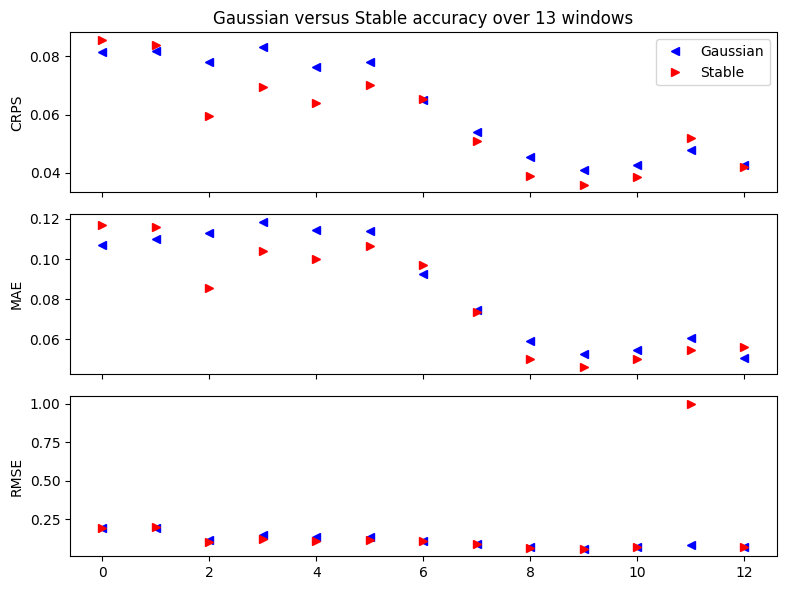
Note that RMSE is a poor metric for evaluating heavy-tailed data. Our stable model has such heavy tails that its variance is infinite, so we cannot expect RMSE to converge, hence occasional outlying points.
[ ]: