高斯过程

高斯过程 (Gaussian Processes ) 可以用于监督，无监督甚至是强化学习的问题中，并由一种优雅的数学理论来描述（有关概述请参见[1，4]）。它们在概念上也很有吸引力，因为它们提供了一种定义 priors over functions 的直观方法。最后，由于高斯过程是在贝叶斯环境下制定的，因此 they come equipped with a powerful notion of uncertainty.

数学理解

高斯过程是基于统计学习理论和贝叶斯理论发展起来的一种机器学习方法，适于处理高维度、小样本和非线性等复杂回归问题，且泛化能力强，与神经网络、支持向量机相比，GP具有容易实现、超参数自适应获取、非参数推断灵活以及输出具有概率意义等优点。See more on 知乎

我尽量避免直接写公式给新接触的人看，多数时候公式可能把创造的动机给掩盖掉，同时让问题是否能 tractable 变得不那么清晰。我想说清楚的是创造工具的动机和背后的问题。那么现在来看看高斯过程方法的动机

平稳高斯过程的一个例子是：

\[X_t = \cos(at)Z_1 + \sin(at)Z_2\]

其中 \(Z_1, Z_2\) 是独立的标准正态分布。那么有几个思考问题：

• \(\mathcal{GP}\left(0, \mathbf{K}_f(x, x')\right)\) 如何与该例子对应？该高斯过程的核函数如何定义？

• 该高斯过程用来近似某个随机函数，那么该随机函数的输入和输出是什么？输入是任意的 \(x'\), 输出是给定 \(x'\) 相关核函数下的过程平稳分布？

• 如何理解 “Ultimately Gaussian processes translate as taking priors on functions and the smoothness of these priors can be induced by the covariance function. If we expect that for”near-by” input points \(x\) and \(x'\) their corresponding output points \(y\) and \(y'\) to be “near-by” also, then the assumption of continuity is present.”

要回答这些问题，建议搜索关键词 Gaussian process prediction, or Kriging

令人高兴的是，Pyro在 pyro.contrib.gp 模块中为高斯过程提供了一些支持。本教程的目的是使用本模块简要介绍高斯过程（GPs）。我们将主要集中于如何在 Pyro 中使用 GP 接口，并向读者介绍有关GP的更多详细信息。

模型定义如下:

\[f \sim \mathcal{GP}\left(0, \mathbf{K}_f(x, x')\right)\]

\[y = f(x) + \epsilon,\quad \epsilon \sim \mathcal{N}\left(0, \beta^{-1}\mathbf{I}\right).\]

其中 \(x, x' \in\mathbf{X}\) 输入空间中的两个点 ，\(y\in\mathbf{Y}\) 是输出空间中的点. \(f\) is a draw from the GP prior specified by the kernel \(\mathbf{K}_f\) and represents a function from \(\mathbf{X}\) to \(\mathbf{Y}\). Finally, \(\epsilon\) represents Gaussian observation noise.

We will use the radial basis function kernel (RBF kernel) as the kernel of our GP:

\[k(x,x') = \sigma^2 \exp\left(-\frac{\|x-x'\|^2}{2l^2}\right).\]

Here \(\sigma^2\) and \(l\) are parameters that specify the kernel; specifically, \(\sigma^2\) is a variance or amplitude squared and \(l\) is a lengthscale. We’ll get some intuition for these parameters below.

数据集

First, we import necessary modules.

import os
import matplotlib.pyplot as plt
import torch

import pyro
import pyro.contrib.gp as gp
import pyro.distributions as dist

smoke_test = ('CI' in os.environ)  # ignore; used to check code integrity in the Pyro repo
assert pyro.__version__.startswith('1.3.0')
pyro.enable_validation(True)       # can help with debugging
pyro.set_rng_seed(0)

Throughout the tutorial we’ll want to visualize GPs. So we define a helper function for plotting:

# note that this helper function does three different things:
# (i) plots the observed data;
# (ii) plots the predictions from the learned GP after conditioning on data;
# (iii) plots samples from the GP prior (with no conditioning on observed data)

def plot(plot_observed_data=False, plot_predictions=False, n_prior_samples=0,
         model=None, kernel=None, n_test=500):

    plt.figure(figsize=(12, 6))
    if plot_observed_data:
        plt.plot(X.numpy(), y.numpy(), 'kx')
    if plot_predictions:
        Xtest = torch.linspace(-0.5, 5.5, n_test)  # test inputs
        # compute predictive mean and variance
        with torch.no_grad():
            if type(model) == gp.models.VariationalSparseGP:
                mean, cov = model(Xtest, full_cov=True)
            else:
                mean, cov = model(Xtest, full_cov=True, noiseless=False)
        sd = cov.diag().sqrt()  # standard deviation at each input point x
        plt.plot(Xtest.numpy(), mean.numpy(), 'r', lw=2)  # plot the mean
        plt.fill_between(Xtest.numpy(),  # plot the two-sigma uncertainty about the mean
                         (mean - 2.0 * sd).numpy(),
                         (mean + 2.0 * sd).numpy(),
                         color='C0', alpha=0.3)
    if n_prior_samples > 0:  # plot samples from the GP prior
        Xtest = torch.linspace(-0.5, 5.5, n_test)  # test inputs
        noise = (model.noise if type(model) != gp.models.VariationalSparseGP
                 else model.likelihood.variance)
        cov = kernel.forward(Xtest) + noise.expand(n_test).diag()
        samples = dist.MultivariateNormal(torch.zeros(n_test), covariance_matrix=cov)\
                      .sample(sample_shape=(n_prior_samples,))
        plt.plot(Xtest.numpy(), samples.numpy().T, lw=2, alpha=0.4)

    plt.xlim(-0.5, 5.5)

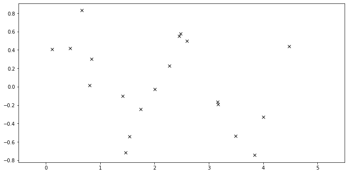
Data

The data consist of \(20\) points sampled from

\[y = 0.5\sin(3x) + \epsilon, \quad \epsilon \sim \mathcal{N}(0, 0.2).\]

with \(x\) sampled uniformly from the interval \([0, 5]\).

N = 20
X = dist.Uniform(0.0, 5.0).sample(sample_shape=(N,))
y = 0.5 * torch.sin(3*X) + dist.Normal(0.0, 0.2).sample(sample_shape=(N,))

plot(plot_observed_data=True)  # let's plot the observed data

构建模型

First we define a RBF kernel, specifying the values of the two hyperparameters variance and lengthscale. Then we construct a GPRegression object. Here we feed in another hyperparameter, noise, that corresponds to \(\epsilon\) above.

kernel = gp.kernels.RBF(input_dim=1, variance=torch.tensor(5.),
                        lengthscale=torch.tensor(10.))
gpr = gp.models.GPRegression(X, y, kernel, noise=torch.tensor(1.))

Let’s see what samples from this GP function prior look like. Note that this is before we’ve conditioned on the data. The shape these functions take—their smoothness, their vertical scale, etc.—is controlled by the GP kernel.

plot(model=gpr, kernel=kernel, n_prior_samples=2)

For example, if we make variance and noise smaller we will see function samples with smaller vertical amplitude:

kernel2 = gp.kernels.RBF(input_dim=1, variance=torch.tensor(0.1),
                         lengthscale=torch.tensor(10.))
gpr2 = gp.models.GPRegression(X, y, kernel2, noise=torch.tensor(0.1))
plot(model=gpr2, kernel=kernel2, n_prior_samples=2)

模型推断和训练

In the above we set the kernel hyperparameters by hand. If we want to learn the hyperparameters from the data, we need to do inference. In the simplest (conjugate) case we do gradient ascent on the log marginal likelihood. In pyro.contrib.gp, we can use any PyTorch optimizer to optimize parameters of a model. In addition, we need a loss function which takes inputs are the pair model and guide and returns an ELBO loss (see SVI Part I tutorial).

optimizer = torch.optim.Adam(gpr.parameters(), lr=0.005)
loss_fn = pyro.infer.Trace_ELBO().differentiable_loss
losses = []
num_steps = 2500 if not smoke_test else 2
for i in range(num_steps):
    optimizer.zero_grad()
    loss = loss_fn(gpr.model, gpr.guide)
    loss.backward()
    optimizer.step()
    losses.append(loss.item())

# Quiz: 都没有数据，如何训练的？数据定义在模型 gpr 之中

-------------------------------------------
NameError Traceback (most recent call last)
<ipython-input-1-97a8bd8ab535> in <module>
----> 1 optimizer = torch.optim.Adam(gpr.parameters(), lr=0.005)
      2 loss_fn = pyro.infer.Trace_ELBO().differentiable_loss
      3 losses = []
      4 num_steps = 2500 if not smoke_test else 2
      5 for i in range(num_steps):

NameError: name 'torch' is not defined

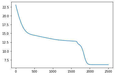
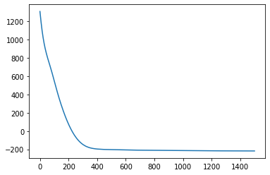
# let's plot the loss curve after 2500 steps of training
plt.plot(losses);

Let’s see if we’re learned anything reasonable:

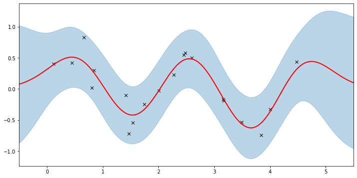
plot(model=gpr, plot_observed_data=True, plot_predictions=True)

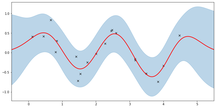
Here the thick red curve is the mean prediction and the blue band represents the 2-sigma uncertainty around the mean. It seems we learned reasonable kernel hyperparameters, as both the mean and uncertainty give a reasonable fit to the data. (Note that learning could have easily gone wrong if we e.g. chose too large of a learning rate or chose bad initital hyperparameters.)

Note that the kernel is only well-defined if variance and lengthscale are positive. Under the hood Pyro is using PyTorch constraints (see docs) to ensure that hyperparameters are constrained to the appropriate domains. Let’s see the constrained values we’ve learned.

gpr.kernel.variance.item()

0.20291335880756378

gpr.kernel.lengthscale.item()

0.5022152662277222

gpr.noise.item()

0.04272938147187233

The period of the sinusoid that generated the data is \(T = 2\pi/3 \approx 2.09\) so learning a lengthscale that’s approximiately equal to a quarter period makes sense.

Fit the model using MAP

We need to define priors for the hyperparameters.

# Define the same model as before.
pyro.clear_param_store()
kernel = gp.kernels.RBF(input_dim=1, variance=torch.tensor(5.),
                        lengthscale=torch.tensor(10.))
gpr = gp.models.GPRegression(X, y, kernel, noise=torch.tensor(1.))

# note that our priors have support on the positive reals
gpr.kernel.lengthscale = pyro.nn.PyroSample(dist.LogNormal(0.0, 1.0))
gpr.kernel.variance = pyro.nn.PyroSample(dist.LogNormal(0.0, 1.0))

optimizer = torch.optim.Adam(gpr.parameters(), lr=0.005)
loss_fn = pyro.infer.Trace_ELBO().differentiable_loss
losses = []
num_steps = 2500 if not smoke_test else 2
for i in range(num_steps):
    optimizer.zero_grad()
    loss = loss_fn(gpr.model, gpr.guide)
    loss.backward()
    optimizer.step()
    losses.append(loss.item())
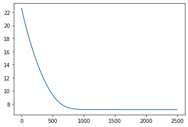
plt.plot(losses);

plot(model=gpr, plot_observed_data=True, plot_predictions=True)

Let’s inspect the hyperparameters we’ve learned:

# tell gpr that we want to get samples from guides
gpr.set_mode('guide')
print('variance = {}'.format(gpr.kernel.variance))
print('lengthscale = {}'.format(gpr.kernel.lengthscale))
print('noise = {}'.format(gpr.noise))

variance = 0.24471399188041687
lengthscale = 0.5217688083648682
noise = 0.04222287982702255

Note that the MAP values are different from the MLE values due to the prior.

稀疏高斯过程

For large datasets computing the log marginal likelihood is costly due to the expensive matrix operations involved (e.g. see Section 2.2 of [1]). A variety of so-called ‘sparse’ variational methods have been developed to make GPs viable for larger datasets. This is a big area of research and we won’t be going into all the details. Instead we quickly show how we can use SparseGPRegression in pyro.contrib.gp to make use of these methods.

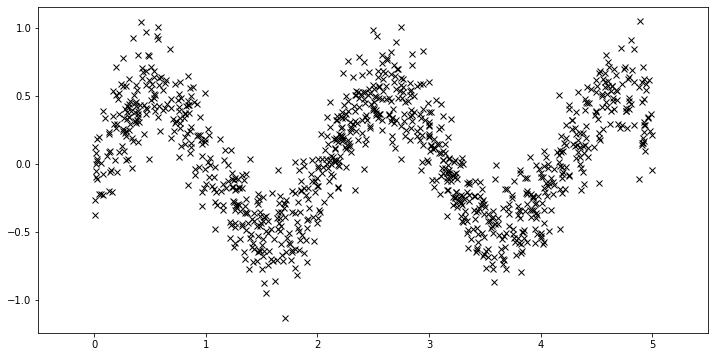
First, we generate more data.

N = 1000
X = dist.Uniform(0.0, 5.0).sample(sample_shape=(N,))
y = 0.5 * torch.sin(3*X) + dist.Normal(0.0, 0.2).sample(sample_shape=(N,))
plot(plot_observed_data=True)

Using the sparse GP is very similar to using the basic GP used above. We just need to add an extra parameter \(X_u\) (the inducing points).

# initialize the inducing inputs
Xu = torch.arange(20.) / 4.0

# initialize the kernel and model
pyro.clear_param_store()
kernel = gp.kernels.RBF(input_dim=1)
# we increase the jitter for better numerical stability
sgpr = gp.models.SparseGPRegression(X, y, kernel, Xu=Xu, jitter=1.0e-5)

# the way we setup inference is similar to above
optimizer = torch.optim.Adam(sgpr.parameters(), lr=0.005)
loss_fn = pyro.infer.Trace_ELBO().differentiable_loss
losses = []
num_steps = 2500 if not smoke_test else 2
for i in range(num_steps):
    optimizer.zero_grad()
    loss = loss_fn(sgpr.model, sgpr.guide)
    loss.backward()
    optimizer.step()
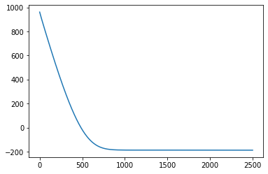
    losses.append(loss.item())
plt.plot(losses);

# let's look at the inducing points we've learned
print("inducing points:\n{}".format(sgpr.Xu.data.numpy()))
# and plot the predictions from the sparse GP
plot(model=sgpr, plot_observed_data=True, plot_predictions=True)

inducing points:
[0.03890638 0.51997566 0.26106593 1.0221936  0.7851976  1.3309097
 1.5923843  1.8223386  2.2960622  2.794138   2.082978   2.5219998
 3.0490053  3.3228474  3.5942013  3.8977344  4.2026505  4.490753
 4.7720113  4.9819574 ]

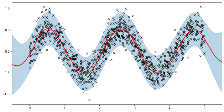
We can see that the model learns a reasonable fit to the data. There are three different sparse approximations that are currently implemented in Pyro:

• “DTC” (Deterministic Training Conditional)

• “FITC” (Fully Independent Training Conditional)

• “VFE” (Variational Free Energy)

By default, SparseGPRegression will use “VFE” as the inference method. We can use other methods by passing a different approx flag to SparseGPRegression.

More Sparse GPs

Both GPRegression and SparseGPRegression above are limited to Gaussian likelihoods. We can use other likelihoods with GPs—for example, we can use the Bernoulli likelihood for classification problems—but the inference problem becomes more difficult. In this section, we show how to use the VariationalSparseGP module, which can handle non-Gaussian likelihoods. So we can compare to what we’ve done above, we’re still going to use a Gaussian likelihood. The point is that the inference that’s being done under the hood can support other likelihoods.

# initialize the inducing inputs
Xu = torch.arange(10.) / 2.0

# initialize the kernel, likelihood, and model
pyro.clear_param_store()
kernel = gp.kernels.RBF(input_dim=1)
likelihood = gp.likelihoods.Gaussian()
# turn on "whiten" flag for more stable optimization
vsgp = gp.models.VariationalSparseGP(X, y, kernel, Xu=Xu, likelihood=likelihood, whiten=True)

# instead of defining our own training loop, we will
# use the built-in support provided by the GP module
num_steps = 1500 if not smoke_test else 2
losses = gp.util.train(vsgp, num_steps=num_steps)
plt.plot(losses);

plot(model=vsgp, plot_observed_data=True, plot_predictions=True)

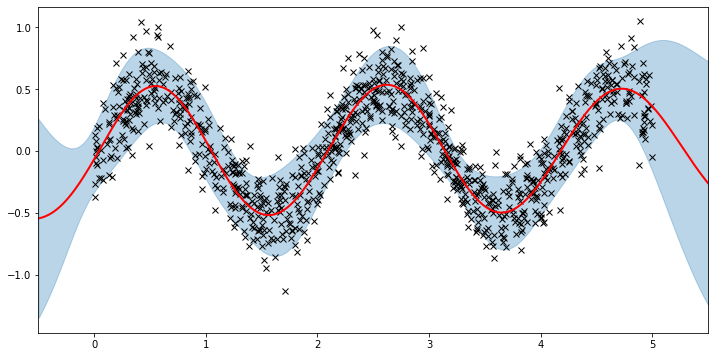
That’s all there is to it. For more details on the pyro.contrib.gp module see the docs. And for example code that uses a GP for classification see here.

参考文献

[1] Deep Gaussian processes and variational propagation of uncertainty,     Andreas Damianou

[2] A unifying framework for sparse Gaussian process approximation using power expectation propagation,     Thang D. Bui, Josiah Yan, and Richard E. Turner

[3] Scalable variational Gaussian process classification,     James Hensman, Alexander G. de G. Matthews, and Zoubin Ghahramani

[4] Gaussian Processes for Machine Learning,     Carl E. Rasmussen, and Christopher K. I. Williams

[5] A Unifying View of Sparse Approximate Gaussian Process Regression,     Joaquin Quinonero-Candela, and Carl E. Rasmussen