贝叶斯回归推断算法(Part II)

在 Part I 中，我们研究了如何使用SVI在简单的贝叶斯线性回归模型上进行推理。在本教程中，we’ll explore more expressive guides as well as exact inference techniques. 我们将使用与以前相同的数据集。

贝叶斯线性回归：我们的目标是再次根据数据集的两个特征预测一个国家的人均 log GDP - whether the nation is in Africa, and its Terrain Ruggedness Index, but we will explore more expressive guides.

+++++ 学完本文，您将看懂如下代码

import logging, os, torch, pyro
import numpy as np
import pandas as pd
import seaborn as sns
import matplotlib.pyplot as plt
import pyro.optim as optim
import pyro.distributions as dist
from torch import nn
from torch.distributions import constraints
from functools import partial
from pyro.nn import PyroModule, PyroSample, Predictive
from pyro.infer import SVI, Trace_ELBO
from pyro.infer.autoguide import AutoDiagonalNormal
pyro.set_rng_seed(1)
assert pyro.__version__.startswith('1.3.0')
%matplotlib inline
plt.style.use('default')
logging.basicConfig(format='%(message)s', level=logging.INFO)
pyro.enable_validation(True)
DATA_URL = "https://d2hg8soec8ck9v.cloudfront.net/datasets/rugged_data.csv"
rugged_data = pd.read_csv(DATA_URL, encoding="ISO-8859-1")

def model(is_cont_africa, ruggedness, log_gdp):
    a = pyro.sample("a", dist.Normal(0., 10.))
    b_a = pyro.sample("bA", dist.Normal(0., 1.))
    b_r = pyro.sample("bR", dist.Normal(0., 1.))
    b_ar = pyro.sample("bAR", dist.Normal(0., 1.))
    sigma = pyro.sample("sigma", dist.Uniform(8.0, 10.))
    mean = a + b_a * is_cont_africa + b_r * ruggedness + b_ar * is_cont_africa * ruggedness
    with pyro.plate("data", len(ruggedness)):
        pyro.sample("obs", dist.Normal(mean, sigma), obs=log_gdp)

def guide(is_cont_africa, ruggedness, log_gdp):
    a_loc = pyro.param('a_loc', torch.tensor(0.))
    a_scale = pyro.param('a_scale', torch.tensor(1.), constraint=constraints.positive)
    sigma_loc = pyro.param('sigma_loc', torch.tensor(1.), constraint=constraints.positive)
    weights_loc = pyro.param('weights_loc', torch.randn(3))
    weights_scale = pyro.param('weights_scale', torch.ones(3), constraint=constraints.positive)

    a = pyro.sample("a", dist.Normal(a_loc, a_scale))
    b_a = pyro.sample("bA", dist.Normal(weights_loc[0], weights_scale[0]))
    b_r = pyro.sample("bR", dist.Normal(weights_loc[1], weights_scale[1]))
    b_ar = pyro.sample("bAR", dist.Normal(weights_loc[2], weights_scale[2]))
    sigma = pyro.sample("sigma", dist.Normal(sigma_loc, torch.tensor(0.05)))
    mean = a + b_a * is_cont_africa + b_r * ruggedness + b_ar * is_cont_africa * ruggedness

svi = SVI(model, guide, optim.Adam({"lr": .05}),loss=Trace_ELBO())
is_cont_africa, ruggedness, log_gdp = train[:, 0], train[:, 1], train[:, 2]
pyro.clear_param_store()
num_iters = 5000 if not smoke_test else 2
for i in range(num_iters):
    elbo = svi.step(is_cont_africa, ruggedness, log_gdp)
    if i % 500 == 0:
        logging.info("Elbo loss: {}".format(elbo))

Elbo loss: 5795.467590510845
Elbo loss: 415.8169444799423
Elbo loss: 250.71916329860687
Elbo loss: 247.19457268714905
Elbo loss: 249.2004036307335
Elbo loss: 250.96484470367432
Elbo loss: 249.35092514753342
Elbo loss: 248.7831552028656
Elbo loss: 248.62140649557114
Elbo loss: 250.4274433851242

num_samples = 1000
predictive = Predictive(model, guide=guide, num_samples=num_samples)
svi_samples = {k: v.reshape(num_samples).detach().cpu().numpy()
               for k, v in predictive(log_gdp, is_cont_africa, ruggedness).items()
               if k != "obs"}
for site, values in summary(svi_samples).items():
    print("Site: {}".format(site))
    print(values, "\n")

Site: a
       mean       std        5%       25%       50%       75%       95%
0  9.177502  0.062302  9.077003  9.134532  9.178522  9.215999  9.278267

Site: bA
       mean       std      5%       25%      50%       75%       95%
0 -1.895068  0.118995 -2.0918 -1.974353 -1.89098 -1.813422 -1.702851

Site: bR
       mean       std        5%       25%       50%       75%       95%
0 -0.157187  0.038121 -0.222267 -0.181703 -0.155021 -0.130235 -0.095558

Site: bAR
       mean       std       5%       25%       50%       75%       95%
0  0.304799  0.066955  0.19294  0.261902  0.304932  0.350269  0.412381

Site: sigma
       mean       std        5%       25%       50%       75%       95%
0  0.902913  0.049275  0.822383  0.870878  0.901005  0.938589  0.983858

Model + Guide

We will write out the model again, similar to that in Part I, but explicitly without the use of PyroModule. We will write out each term in the regression, using the same priors. bA and bR are regression coefficients corresponding to is_cont_africa and ruggedness, a is the intercept, and bAR is the correlating factor between the two features.

Writing down a guide will proceed in close analogy to the construction of our model, with the key difference that the guide parameters need to be trainable. To do this we register the guide parameters in the ParamStore using pyro.param(). Note the positive constraints on scale parameters.

# Utility function to print latent sites' quantile information.
def summary(samples):
    site_stats = {}
    for site_name, values in samples.items():
        marginal_site = pd.DataFrame(values)
        describe = marginal_site.describe(percentiles=[.05, 0.25, 0.5, 0.75, 0.95]).transpose()
        site_stats[site_name] = describe[["mean", "std", "5%", "25%", "50%", "75%", "95%"]]
    return site_stats

# Prepare training data
df = rugged_data[["cont_africa", "rugged", "rgdppc_2000"]]
df = df[np.isfinite(df.rgdppc_2000)]
df["rgdppc_2000"] = np.log(df["rgdppc_2000"])
train = torch.tensor(df.values, dtype=torch.float)

SVI

As before, we will use SVI to perform inference.

from pyro.infer import SVI, Trace_ELBO


svi = SVI(model, guide, optim.Adam({"lr": .05}),loss=Trace_ELBO())

is_cont_africa, ruggedness, log_gdp = train[:, 0], train[:, 1], train[:, 2]
pyro.clear_param_store()
num_iters = 5000 if not smoke_test else 2
for i in range(num_iters):
    elbo = svi.step(is_cont_africa, ruggedness, log_gdp)
    if i % 500 == 0:
        logging.info("Elbo loss: {}".format(elbo))

Elbo loss: 5795.467590510845
Elbo loss: 415.8169444799423
Elbo loss: 250.71916329860687
Elbo loss: 247.19457268714905
Elbo loss: 249.2004036307335
Elbo loss: 250.96484470367432
Elbo loss: 249.35092514753342
Elbo loss: 248.7831552028656
Elbo loss: 248.62140649557114
Elbo loss: 250.4274433851242

from pyro.infer import Predictive

num_samples = 1000
predictive = Predictive(model, guide=guide, num_samples=num_samples)
svi_samples = {k: v.reshape(num_samples).detach().cpu().numpy()
               for k, v in predictive(log_gdp, is_cont_africa, ruggedness).items()
               if k != "obs"}

Let us observe the posterior distribution over the different latent variables in the model.

for site, values in summary(svi_samples).items():
    print("Site: {}".format(site))
    print(values, "\n")

Site: a
      mean       std       5%       25%       50%       75%      95%
0  9.17702  0.059607  9.07811  9.140463  9.178211  9.217098  9.27152

Site: bA
       mean       std       5%       25%       50%       75%       95%
0 -1.890622  0.122805 -2.08849 -1.979107 -1.887476 -1.803683 -1.700853

Site: bR
       mean       std       5%       25%       50%       75%       95%
0 -0.157847  0.039538 -0.22324 -0.183673 -0.157873 -0.133102 -0.091713

Site: bAR
       mean       std        5%       25%       50%       75%       95%
0  0.304515  0.067683  0.194583  0.259464  0.304907  0.348932  0.415128

Site: sigma
       mean       std        5%       25%       50%       75%       95%
0  0.902898  0.047971  0.824166  0.870317  0.901981  0.935171  0.981577

HMC

In contrast to using variational inference which gives us an approximate posterior over our latent variables, we can also do exact inference using Markov Chain Monte Carlo (MCMC), a class of algorithms that in the limit, allow us to draw unbiased samples from the true posterior. The algorithm that we will be using is called the No-U Turn Sampler (NUTS) [1], which provides an efficient and automated way of running Hamiltonian Monte Carlo. It is slightly slower than variational inference, but provides an exact estimate.

from pyro.infer import MCMC, NUTS


nuts_kernel = NUTS(model)

mcmc = MCMC(nuts_kernel, num_samples=1000, warmup_steps=200)
mcmc.run(is_cont_africa, ruggedness, log_gdp)

hmc_samples = {k: v.detach().cpu().numpy() for k, v in mcmc.get_samples().items()}

Sample: 100%|██████████| 1200/1200 [00:30, 38.99it/s, step size=2.76e-01, acc. prob=0.934]

for site, values in summary(hmc_samples).items():
    print("Site: {}".format(site))
    print(values, "\n")

Site: a
       mean      std        5%       25%       50%       75%       95%
0  9.182098  0.13545  8.958712  9.095588  9.181347  9.277673  9.402615

Site: bA
       mean       std       5%       25%       50%      75%       95%
0 -1.847651  0.217768 -2.19934 -1.988024 -1.846978 -1.70495 -1.481822

Site: bR
       mean       std        5%       25%       50%       75%       95%
0 -0.183031  0.078067 -0.311403 -0.237077 -0.185945 -0.131043 -0.051233

Site: bAR
       mean       std        5%       25%      50%       75%       95%
0  0.348332  0.127478  0.131907  0.266548  0.34641  0.427984  0.560221

Site: sigma
       mean       std        5%       25%       50%       75%       95%
0  0.952041  0.052024  0.869388  0.914335  0.949961  0.986266  1.038723

Comparing Posterior Distributions

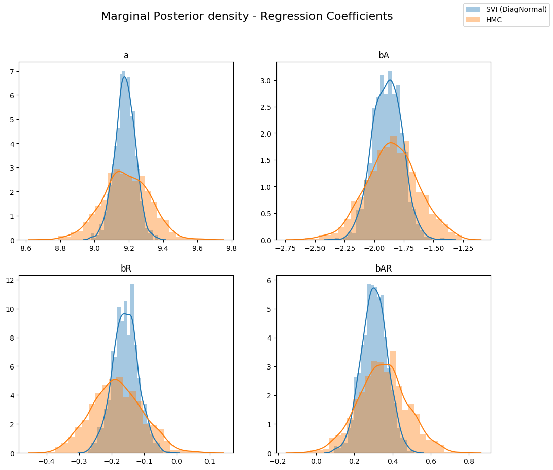
Let us compare the posterior distribution of the latent variables that we obtained from variational inference with those from Hamiltonian Monte Carlo. As can be seen below, for Variational Inference, the marginal distribution of the different regression coefficients is under-dispersed w.r.t. the true posterior (from HMC). This is an artifact of the KL(q||p) loss (the KL divergence of the true posterior from the approximate posterior) that is minimized by Variational Inference.

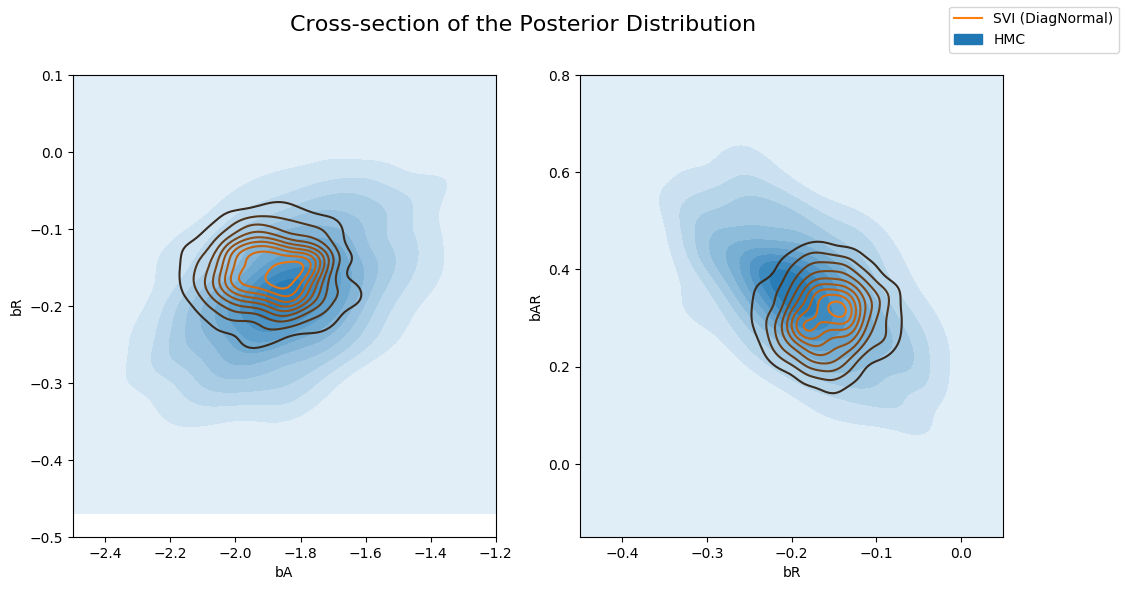
This can be better seen when we plot different cross sections from the joint posterior distribution overlaid with the approximate posterior from variational inference. Note that since our variational family has diagonal covariance, we cannot model any correlation between the latents and the resulting approximation is overconfident (under-dispersed)

sites = ["a", "bA", "bR", "bAR", "sigma"]

fig, axs = plt.subplots(nrows=2, ncols=2, figsize=(12, 10))
fig.suptitle("Marginal Posterior density - Regression Coefficients", fontsize=16)
for i, ax in enumerate(axs.reshape(-1)):
    site = sites[i]
    sns.distplot(svi_samples[site], ax=ax, label="SVI (DiagNormal)")
    sns.distplot(hmc_samples[site], ax=ax, label="HMC")
    ax.set_title(site)
handles, labels = ax.get_legend_handles_labels()
fig.legend(handles, labels, loc='upper right');

fig, axs = plt.subplots(nrows=1, ncols=2, figsize=(12, 6))
fig.suptitle("Cross-section of the Posterior Distribution", fontsize=16)
sns.kdeplot(hmc_samples["bA"], hmc_samples["bR"], ax=axs[0], shade=True, label="HMC")
sns.kdeplot(svi_samples["bA"], svi_samples["bR"], ax=axs[0], label="SVI (DiagNormal)")
axs[0].set(xlabel="bA", ylabel="bR", xlim=(-2.5, -1.2), ylim=(-0.5, 0.1))
sns.kdeplot(hmc_samples["bR"], hmc_samples["bAR"], ax=axs[1], shade=True, label="HMC")
sns.kdeplot(svi_samples["bR"], svi_samples["bAR"], ax=axs[1], label="SVI (DiagNormal)")
axs[1].set(xlabel="bR", ylabel="bAR", xlim=(-0.45, 0.05), ylim=(-0.15, 0.8))
handles, labels = axs[1].get_legend_handles_labels()
fig.legend(handles, labels, loc='upper right');

MultivariateNormal Guide

As comparison to the previously obtained results from Diagonal Normal guide, we will now use a guide that generates samples from a Cholesky factorization of a multivariate normal distribution. This allows us to capture the correlations between the latent variables via a covariance matrix. If we wrote this manually, we would need to combine all the latent variables so we could sample a Multivarite Normal jointly.

from pyro.infer.autoguide import AutoMultivariateNormal, init_to_mean


guide = AutoMultivariateNormal(model, init_loc_fn=init_to_mean)

svi = SVI(model,
          guide,
          optim.Adam({"lr": .01}),
          loss=Trace_ELBO())

is_cont_africa, ruggedness, log_gdp = train[:, 0], train[:, 1], train[:, 2]
pyro.clear_param_store()
for i in range(num_iters):
    elbo = svi.step(is_cont_africa, ruggedness, log_gdp)
    if i % 500 == 0:
        logging.info("Elbo loss: {}".format(elbo))

Elbo loss: 703.0100790262222
Elbo loss: 444.6930855512619
Elbo loss: 258.20718491077423
Elbo loss: 249.05364602804184
Elbo loss: 247.2170884013176
Elbo loss: 247.28261297941208
Elbo loss: 246.61236548423767
Elbo loss: 249.86004841327667
Elbo loss: 249.1157277226448
Elbo loss: 249.86634194850922

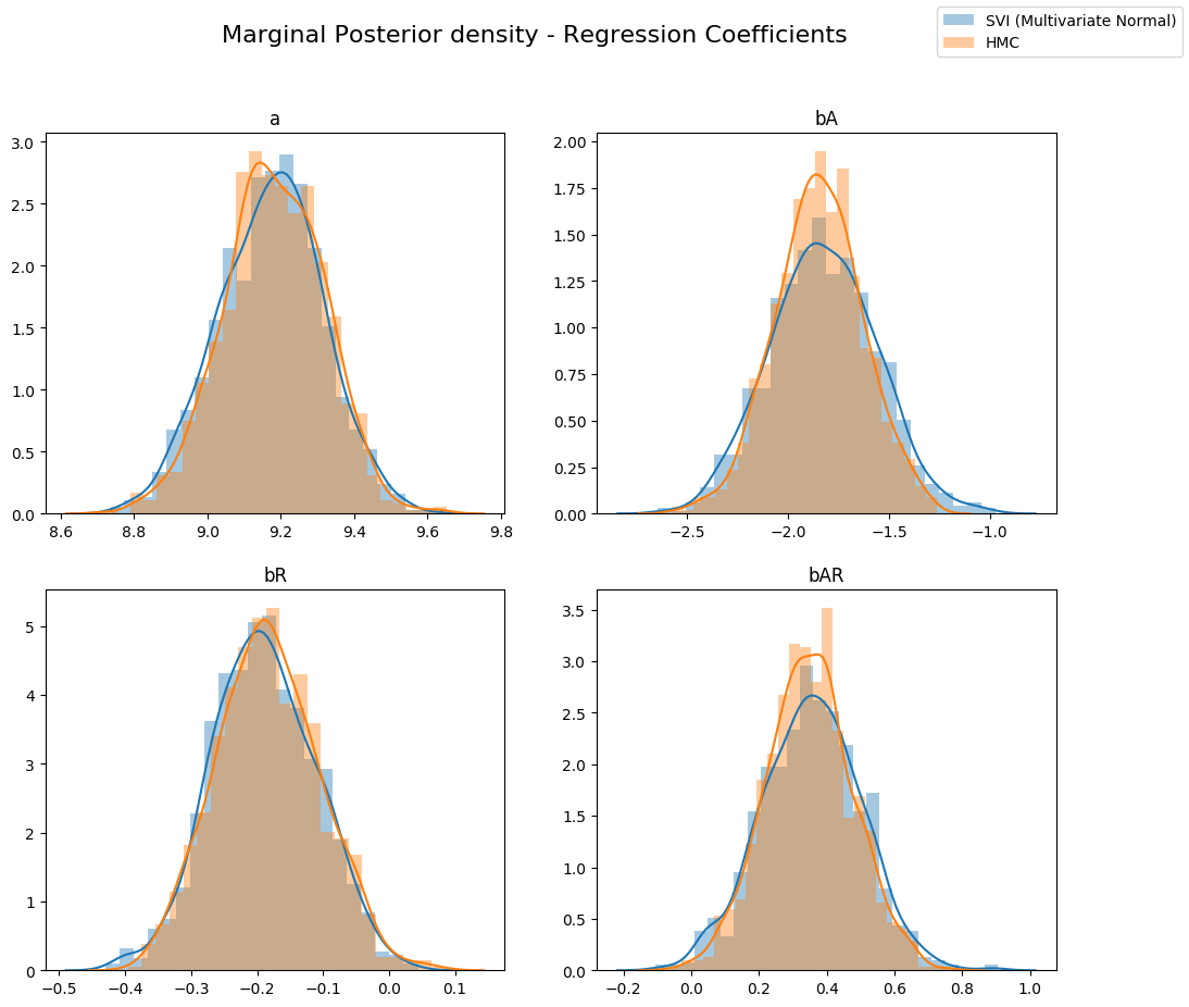
Let’s look at the shape of the posteriors again. You can see the multivariate guide is able to capture more of the true posterior.

predictive = Predictive(model, guide=guide, num_samples=num_samples)
svi_mvn_samples = {k: v.reshape(num_samples).detach().cpu().numpy()
                   for k, v in predictive(log_gdp, is_cont_africa, ruggedness).items()
                   if k != "obs"}
fig, axs = plt.subplots(nrows=2, ncols=2, figsize=(12, 10))
fig.suptitle("Marginal Posterior density - Regression Coefficients", fontsize=16)
for i, ax in enumerate(axs.reshape(-1)):
    site = sites[i]
    sns.distplot(svi_mvn_samples[site], ax=ax, label="SVI (Multivariate Normal)")
    sns.distplot(hmc_samples[site], ax=ax, label="HMC")
    ax.set_title(site)
handles, labels = ax.get_legend_handles_labels()
fig.legend(handles, labels, loc='upper right');

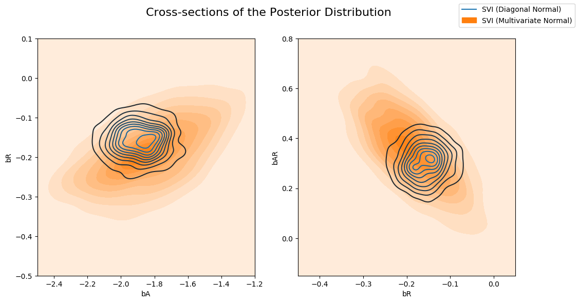
Now let’s compare the posterior computed by the Diagonal Normal guide vs the Multivariate Normal guide. Note that the multivariate distribution is more dispresed than the Diagonal Normal.

fig, axs = plt.subplots(nrows=1, ncols=2, figsize=(12, 6))
fig.suptitle("Cross-sections of the Posterior Distribution", fontsize=16)
sns.kdeplot(svi_samples["bA"], svi_samples["bR"], ax=axs[0], label="HMC")
sns.kdeplot(svi_mvn_samples["bA"], svi_mvn_samples["bR"], ax=axs[0], shade=True, label="SVI (Multivariate Normal)")
axs[0].set(xlabel="bA", ylabel="bR", xlim=(-2.5, -1.2), ylim=(-0.5, 0.1))
sns.kdeplot(svi_samples["bR"], svi_samples["bAR"], ax=axs[1], label="SVI (Diagonal Normal)")
sns.kdeplot(svi_mvn_samples["bR"], svi_mvn_samples["bAR"], ax=axs[1], shade=True, label="SVI (Multivariate Normal)")
axs[1].set(xlabel="bR", ylabel="bAR", xlim=(-0.45, 0.05), ylim=(-0.15, 0.8))
handles, labels = axs[1].get_legend_handles_labels()
fig.legend(handles, labels, loc='upper right');

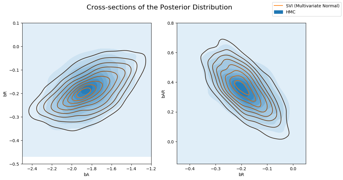
and the Multivariate guide with the posterior computed by HMC. Note that the Multivariate guide better captures the true posterior.

fig, axs = plt.subplots(nrows=1, ncols=2, figsize=(12, 6))
fig.suptitle("Cross-sections of the Posterior Distribution", fontsize=16)
sns.kdeplot(hmc_samples["bA"], hmc_samples["bR"], ax=axs[0], shade=True, label="HMC")
sns.kdeplot(svi_mvn_samples["bA"], svi_mvn_samples["bR"], ax=axs[0], label="SVI (Multivariate Normal)")
axs[0].set(xlabel="bA", ylabel="bR", xlim=(-2.5, -1.2), ylim=(-0.5, 0.1))
sns.kdeplot(hmc_samples["bR"], hmc_samples["bAR"], ax=axs[1], shade=True, label="HMC")
sns.kdeplot(svi_mvn_samples["bR"], svi_mvn_samples["bAR"], ax=axs[1], label="SVI (Multivariate Normal)")
axs[1].set(xlabel="bR", ylabel="bAR", xlim=(-0.45, 0.05), ylim=(-0.15, 0.8))
handles, labels = axs[1].get_legend_handles_labels()
fig.legend(handles, labels, loc='upper right');

参考文献

[1] Hoffman, Matthew D., and Andrew Gelman. “The No-U-turn sampler: adaptively setting path lengths in Hamiltonian Monte Carlo.” Journal of Machine Learning Research 15.1 (2014): 1593-1623. https://arxiv.org/abs/1111.4246.